What is the Dynamic Range of a Receiver?
Since the term dynamic range is often used when discussing the performance of a receiver, it is important to clearly understand what it refers to and its practical significance.
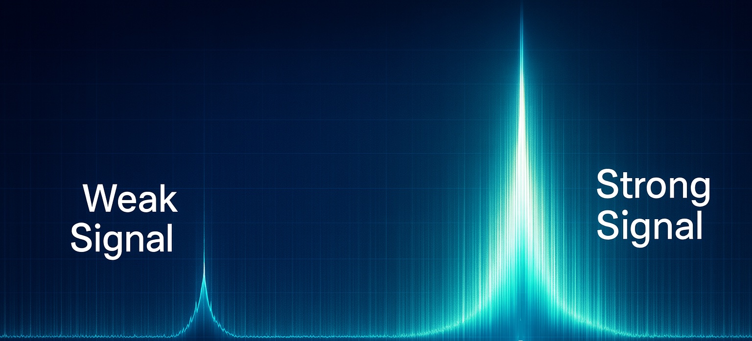
Imagine listening to sounds ranging from a very soft whisper to a loud, intense noise. If you can hear both clearly, without the loud sound overwhelming you or the soft one disappearing, then your hearing has a wide dynamic range.
The greater this distance, meaning the difference in intensity between the weakest and the strongest sound you can perceive without distortion, the larger your dynamic range is.
The same applies to a receiver. At one end lies the weakest signal it can detect without being lost in noise, and at the other the strongest signal it can accept without causing distortion.
The difference between these two extremes defines the dynamic range of the receiver.
Contents
Example:
Imagine that you are using a receiver.
If its dynamic range is limited:
- Weak stations will either not be heard at all or will be received with noise and poor quality.
- Very strong stations may cause distortion in the audio, resulting in a harsh, noisy, and unpleasant signal.
In contrast, if the dynamic range is wide:
- You will be able to receive distant and weak stations with clarity and detail.
- Strong stations will not overload or saturate the receiver, maintaining a clean and stable sound.
Overall, a receiver with a wide dynamic range provides cleaner, more flexible, and more reliable performance, even under challenging radio communication conditions.
How is dynamic range measured?
Dynamic range is measured in decibels (dB), a logarithmic quantity that expresses the ratio between the strongest and the weakest signal a receiver can handle without distortion or loss.
- A simple, basic receiver may have a dynamic range around 60 to 70 dB.
- A high-quality, professional receiver can reach or even exceed 100 dB.
The larger this value is, the better the receiver can handle signals of very different intensities, “perceive” weak ones without being suppressed by strong ones, and avoid distortion.
Imagine listening to sounds ranging from a very soft whisper to a loud, intense noise. If you can hear both clearly, without the loud sound overwhelming you or the soft one disappearing, then your hearing has a wide dynamic range.
In areas with many transmitters or with weak signals, a receiver with a high dynamic range is essential so that:
- All stations are received clearly.
- Weak stations are not masked by stronger ones.
- Reception remains stable, clean, and reliable.
Having provided a general and simplified picture of what a receiver’s dynamic range is, we can now proceed to a more detailed examination of this characteristic and look at its technical aspects in greater depth.
Dynamic Range – In Detail
The Dynamic Range (DR) of a receiver is defined as the difference, in decibels (dB), between the strongest signal it can accept without causing significant distortion (usually at the compression point or the IP3 limit) and the weakest signal it can detect with an acceptable signal-to-noise ratio (SNR).
The mathematical expression of dynamic range is:
DR = Pmax usable − Pmin detectable
Where:
- Pmax usable: the power of the strongest signal without distortion (usually before compression or intermodulation).
- Pmin detectable: the minimum discernible signal power (MDS – Minimum Discernible Signal).
In practice, dynamic range can be divided into three main types.
A. Spurious-Free Dynamic Range (SFDR)
The Spurious-Free Dynamic Range (SFDR) is a critical parameter in evaluating the performance of conventional RF receivers as well as digital receivers such as SDRs (Software Defined Radios). It defines the range of input signal levels within which the receiver can detect and process signals without the occurrence of unwanted distortions, such as third-order intermodulation products (IMD3) or other spurious components.
Definition and Calculation
The SFDR is determined by the difference, in dB, between the signal level and the strongest distortion product or the noise, whichever is closer in level:
SFDR = ⅔ ( IP3 – Noise Floor )
Where:
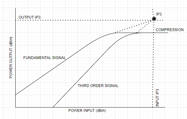
- IP3 (Third-Order Intercept Point):
The IP3 is the point at which the power of the third-order intermodulation products would (theoretically) converge with the power of the fundamental signal if their curves were extended linearly.
- In RF (Radio Frequency) systems in general, the linear operation of amplifiers and other active components is critical for the accurate transmission and reception of signals. However, when the level of the desired signal increases and approaches a certain limit, known as the Third-Order Intercept Point or IP3, nonlinear effects begin to appear, leading to distortion.
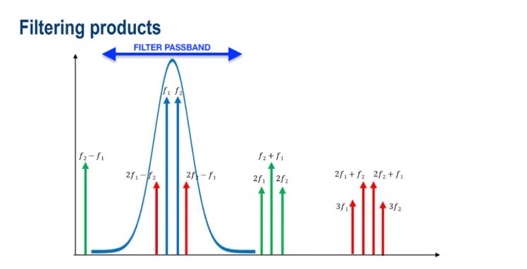
- Suppose you have two input signals with frequencies f1 and f2
An ideal (linear) system would process these signals without generating new frequencies. However, a nonlinear system (such as a high-power amplifier operating near saturation) introduces harmonics and intermodulation due to its nonlinear characteristics.
The output of the nonlinear system can be expressed with a Taylor series, which ultimately produces third-order intermodulation products such as 2f1 − f2, 2f2 − f1, 3f1, 3f2, f1 + f2, and others.
Among these, the most critical (worst) third-order products are:
2f1 − f2 and 2f2 − f1
These products are especially problematic because they fall very close to the original frequencies f₁ and f₂, making effective separation or filtering extremely difficult. As a result, they can cause interference with the desired signal, degrading reception quality and overall system performance.
- Understanding and calculating IP3 is therefore essential in the design and evaluation of RF circuits, particularly in applications where high linearity is required, such as in wireless communications, satellite systems, and broadband networks.
- Noise Floor:
This is the lowest noise level of a system, meaning the minimum signal level below which the signal is “lost” within the noise. It is usually expressed in dBm and depends on factors such as thermal radiation, system gain, and the noise of electronic circuits.
B. Blocking Dynamic Range (BDR)
The Blocking Dynamic Range (BDR) expresses the ability of the receiver to detect a weak signal in the presence of a strong interfering signal (“blocking signal”), either on an adjacent frequency or in a more distant out-of-band region.
It is defined as:
BDR = Pblocking − Pmin detectable
Where:
- Pblocking: The maximum level of the strong signal that does not affect the reception of the weak signal.
- Pmin detectable: The minimum detectable signal power (Minimum Detectable Signal – MDS).
Technical Significance
Blocking Dynamic Range (BDR) expresses the resilience of the receiver’s front-end against saturation caused by strong out-of-band signals. It is a critical performance indicator, especially in environments with strong interference. BDR is mainly influenced by:
- The linearity of the first low-noise amplifier (LNA), which determines how well the receiver can tolerate strong signals without introducing distortion.
- The behavior of the mixer under strong-signal conditions, particularly regarding third-order intermodulation products.
- The operation of the AGC (Automatic Gain Control) which can either improve the receiver’s response to high signal levels or limit performance if it does not adapt properly.
A high BDR indicates that the receiver can operate reliably in an environment with strong interference without degrading the reception of weak signals.
Let’s see what Receiver Saturation is
Saturation in a receiver is the condition in which the circuit can no longer amplify the input signals linearly due to excessively high input power.
Under normal operating conditions, the receiver (and especially its first stage, the low-noise amplifier – LNA) amplifies the input signals linearly, meaning the output power is proportional to the input power.
However, when the input signal becomes too strong, the circuit reaches its physical limits. The output stops increasing proportionally, resulting in signal distortion.
What are the consequences of saturation?
- Loss of signal quality: the desired signal is distorted.
- Generation of spurious frequencies: unwanted intermodulation products appear.
- Reduced performance: the receiver may become “confused” and fail to properly distinguish the signal from noise or interference.
- Inability to receive weak signals: when the receiver is “flooded” by a strong signal, it cannot detect weak ones. This is also called blocking.
How can we avoid saturation?
- By using Attenuators for very strong signals.
- By using AGC (Automatic Gain Control) for automatic gain adjustment.
- By selecting high-quality amplifiers with a wide dynamic range.
C. Reciprocal Mixing Dynamic Range (RMDR)
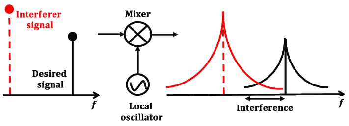
Reciprocal Mixing Dynamic Range (RMDR) expresses the ability of the receiver to detect a weak signal in the presence of a strong adjacent signal (for example, from a nearby transmitter), whose spectral skirts are caused by the phase noise of the local oscillator (LO phase noise).
Let’s explain this simply and clearly.
Phase noise is an unwanted type of fluctuation in the phase of an oscillator or frequency generator’s signal. Instead of being a perfectly clean sine wave at a fixed frequency, the signal exhibits small random “fluctuations” (jitter) around that frequency. On a spectrum analyzer, these appear as noise around the carrier.
How is phase noise measured?
The unit for phase noise is dBc/Hz (decibels relative to the carrier per Hertz). It shows how much lower (in dB) the noise power is compared to the carrier power within a 1 Hz bandwidth, at a specific offset from the carrier frequency.
For example, phase noise of −139 dBc/Hz @ 1 kHz offset means:
- At a frequency 1 kHz away from the oscillator’s carrier, the phase noise is −139 dBc/Hz.
- In other words, at a distance of 1 kHz from the oscillator’s carrier frequency, the noise power is 139 dB lower than the carrier power, at a bandwidth of 1 Hz.
The phase instability of the local oscillator (LO) leads to reciprocal mixing, in which noise from the strong signal “leaks” into the spectrum of the weak signal, degrading the signal-to-noise ratio (SNR) and therefore the quality of reception.
Technical Significance
A high RMDR indicates:
- Good LO quality with low phase noise, especially close to the carrier.
- Increased ability to suppress interference from strong adjacent transmitters.
It is a critical parameter in HF/VHF environments with dense spectral occupancy (for example, amateur contests, HF SDR with multiple simultaneous transmissions, CW, radar).
…a receiver with a wide dynamic range provides cleaner, more flexible, and more reliable performance, even under challenging radio communication conditions.
Factors Affecting Receiver Dynamic Range
Let us now look at the main factors that affect the dynamic range of a receiver:
- Input Noise (Noise Figure – NF):
The input noise represents the degradation of the signal-to-noise ratio (SNR) caused by the receiver itself. It is a fundamental parameter in determining the sensitivity of the system, directly influencing the lower limit of detectable signal (Minimum Detectable Signal – MDS). The lower the NF, the better the receiver’s ability to detect weak signals in high-noise environments.
- Linearity (IP3/IP2, 1 dB Compression Point):
Linearity defines the ability of the receiver to handle strong signals without introducing nonlinear distortions. Parameters such as the third- and second-order intercept points (IP3/IP2) and the 1 dB Compression Point set the gain limits beyond which the system response deviates from linear behavior, affecting the accuracy and clarity of the received signal.
Let us digress to see exactly what the 1 dB Compression Point and IP2 are.
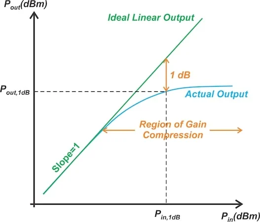
- The 1 dB Compression Point is the input signal power level at which the receiver’s gain drops by 1 dB compared to the ideal, linear gain.
What this means in practice:
- In ideal, linear operation, the output of the amplifier increases proportionally with the input.
However, when the input signal power becomes too large, the circuit enters saturation due to the physical limitations of its components.
At this point (the 1 dB Compression Point), the output no longer increases linearly and begins to “compress.”
It is called the “1 dB” Compression Point because the output is 1 dB lower than what would be expected if the system had remained linear.
- The IP2 (Second-Order Intercept Point) is a theoretical point where the power level of second-order intermodulation products would equal the power level of the original signal if both increased linearly. It is measured in dBm and is not an actual operating point, but rather a way to quantify the nonlinearity of the receiver.
Second-order products appear when two signals of different frequencies f1 and f2 enter a nonlinear amplifier or mixer, generating new signals at the frequencies:
f1 + f2 and | f1 − f2 |
In particular, if f1 − f2 falls within the band of interest (that is, where we expect “clean” signals), it can cause interference.
If the IP2 power level is low, distortion is higher and the ability to distinguish signals is reduced.
If the IP2 power level is high, linearity is better and fewer unwanted signals are produced.
Example:
If a receiver has an IP2 value of +20 dBm, this means that the second-order products will reach the same power level as the main signal when the input signal power theoretically reaches +20 dBm. At this point, significant distortion will occur. Therefore, the higher the IP2 value, the “cleaner” the system operation, since it maintains better linearity at lower input signal power levels.
This concludes the digression.

- Local Oscillator (LO) Phase Noise:
When a strong out-of-band signal is present, the phase noise of the LO “spreads” part of its power into the spectrum around the tuning frequency.
The result is that this strong signal “mixes” (reciprocal mixing) with the LO noise and creates interference within the band of interest.
As a consequence, the noisy background (noise floor) around the desired frequency increases, reducing the receiver’s ability to distinguish weak signals close to strong ones.
Simply put:
High phase noise of the local oscillator (LO) reduces the RMDR, because it increases the unwanted noise at the receive frequency, degrading both the selectivity and sensitivity of the receiver. - ADC Resolution (Bit Depth – ENOB, Effective Number of Bits)
In SDR receivers, the bit depth is the number of bits used by the ADC (Analog-to-Digital Converter) to represent the amplitude of each sample. This characteristic determines the accuracy of the digital representation of the analog signal and directly affects the dynamic range of the receiver. A greater bit depth results in a higher dynamic range and better performance in environments with strong noise or interference.
The Effective Number of Bits (ENOB) is an indicator that measures the actual performance of an ADC, expressing how many “useful” bits of information it delivers in practice. Its calculation takes into account noise, distortion, and other non-ideal system parameters.
ENOB is usually derived from the measurement of SINAD (Signal-to-Noise and Distortion Ratio), using the following formula:
ENOB = SINAD−1.76dB / 6.02dB
SINAD is expressed in dB and includes both noise and distortion.
The number 6.02 comes from the theoretical relation that 1 bit corresponds to approximately 6.02 dB of dynamic range.
The constant 1.76 dB results from the mathematical analysis of uniform quantization noise in an ideal ADC, where it is assumed that noise is uniformly distributed and that 100% of the signal is utilized.
The ENOB essentially defines how cleanly and reliably a signal can be analyzed in an SDR or other digital system. - Automatic Gain Control (AGC):
The AGC dynamically adjusts the gain of the signal so that it remains within the receiver’s optimal operating level, preventing both saturation and excessive attenuation. In this way, stable signal quality is ensured regardless of variations in the input signal power.
…a receiver designed for amateur radio contest use or for high-interference (QRM) environments should have a dynamic range greater than 100 dB in order to handle the simultaneous presence of strong and weak signals effectively.
High-Performance Receiver Evaluation Table
| PARAMETER | TYPICAL VALUE | COMMENT |
|---|---|---|
| SFDR (Spurious-Free Dynamic Range) | ≥ 100 dB | Very good for systems requiring extremely low noise and minimal spurious responses. Values ≥ 100 dB are considered excellent for high-end receivers. |
| BDR (Blocking Dynamic Range) | ≥100–110 dB | Very good value, especially for a narrowband receiver. If it is wideband, it may be more difficult to achieve. |
| RMDR (Reciprocal Mixing Dynamic Range) | ≥ 100 dB @ 2–5 kHz offset | Very good value. RMDR is affected by the phase noise of the local oscillator. Values ≥ 100 dB are excellent for short-range off-channel interference. |
| MDS (Minimum Detectable Signal) | ≤ –130 dBm (in narrowband) | Very sensitive receiver. Achievable in narrowband with filters and low noise. For comparison, –130 dBm corresponds to SNR ≈ 0 dB in a very narrow bandwidth (e.g., 500 Hz). |
| IP3 (Third-Order Intercept Point) | ≥ +10 dBm | Adequate for many receivers. In highly demanding RF environments (e.g., radar), ≥ +20 dBm may be required. |
Question: Can we improve the Dynamic Range of a Receiver?
Answer: YES
The dynamic range of a receiver can be significantly improved through proper design and careful component selection. Below are key ways to improve it.
1. Use of Preselection Filters
They limit the input spectrum by rejecting unwanted out-of-band signals, reducing the likelihood of saturation and improving the Blocking Dynamic Range (BDR).
2. Integration of Low Noise Amplifiers (LNAs)
LNAs are placed at the input of the receive chain to amplify very low-level signals while minimizing additional noise contribution. In this way, the overall sensitivity of the receiver is improved and the minimum detectable signal (MDS) is reduced, enabling the reliable detection and processing of weak signals.
3. Optimized Mixers and Intermediate Frequency (IF) Filters
The use of linear mixers and selective IF filters enhances linearity and selectivity, contributing to higher SFDR and RMDR.
4. Effective Automatic Gain Control (AGC)
Maintains signal levels within the optimal operating range, preventing saturation and improving the overall dynamic behavior of the receiver.
…a good receiver is not simply one that “hears far,” but one that can detect very weak signals, withstand strong interference, and maintain signal integrity without distortion or loss of information.
Conclusions
A high-quality receiver must have the largest possible dynamic range, as this is a decisive factor for its overall performance in realistic, noisy Radio Frequency (RF) environments.
In such environments, both coexist:
- Weak signals, which must not be lost in system noise.
- Strong signals, which must not cause distortion or saturation of the front end.
For example, a receiver designed for amateur radio contest use or for high-interference (QRM) environments should have a dynamic range greater than 100 dB in order to handle the simultaneous presence of strong and weak signals effectively.
Therefore, a good receiver is not simply one that “hears far,” but one that can detect very weak signals, withstand strong interference, and maintain signal integrity without distortion or loss of information.
This is why, when selecting a receiver, it is important to evaluate not only its sensitivity but also its ability to operate in complex RF environments. This capability is reflected in the dynamic range, which is a fundamental indicator of quality and performance.
The same applies to professional measurement instruments, such as spectrum analyzers and network analyzers, where a high dynamic range is essential for accurate and reliable measurements.
…when selecting a receiver, it is important to evaluate not only its sensitivity but also its ability to operate in complex RF environments. This capability is reflected in the dynamic range, which is a fundamental indicator of quality and performance.
It is worth noting that increasing dynamic range entails a significant increase in cost. Devices with a dynamic range above 100 dB are often many times more expensive than those with 60–70 dB, with the price difference often disproportionately large compared to the performance improvement.
Understanding dynamic range is essential for appreciating how receivers perform in real-world RF environments. Whether you are a casual listener, an SDR enthusiast, or a serious contester, knowing what dynamic range is, how it is measured, and how it affects you will help you make better choices and get the most out of your equipment. At the end of the day, it is this balance between sensitivity and resilience that makes the difference in pulling that weak signal out of the noise.