Written by Kostas Stamatis, SV1DPI
Carl Luetzelschwab, K9LA back in 2004, wrote an article called “An Introductory Tutorial to W6ELProp – Running Your Own Propagation Predictions”. This file helped me a lot to understand how w6elprop works and use it more effectively. I made this page mainly to help Greek hams who don’t know English to understand the w6el program. After some thought, I translated my page to English.
W6ELprop is written by W6EL. It helps us make our own predictions of propagation. This program continues in windows what miniprop did in DOS and the author offers it free of charge.
You can download the program at W6EL’s website. You will see at the bottom of the page with red letters “Download W6ELprop v2.70″.
Click and download the program. Run and install it, following the guide. Because that page gives an error sometimes, you can also download it from my site.
Initial Settings
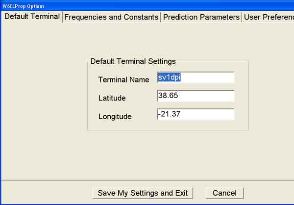
When you finish the installation, run the program and click on “Options“. You will see a window like the one below, saying on the top left “Default Terminal“. Enter your Callsign, Latitude and Longitude. Have in mind that if you are East or South you must add a minus to show it. For example I am 38.65 North and 21.37 East and I wrote what you see below.
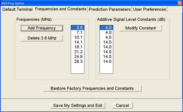
After this, go to the second tab called “Frequencies and Constants“. Here you can add the frequencies you are interested in. Let’s say you want to make predictions for 3.7, 7.1, 10.1, 14.2, 18.1, 21.2, 24.9 and 28.3. Click where it says “Add Frequency“. So you can add a frequency in MHz (you must write 18.1 and not 18100 for 17m). Have in mind that we can not make predictions below 3.5 or above 30 MHz. For 160m you can use 80m predictions as a start.
On the right you will see “Additive Signal Level Constants (dB)”. We can add our station data here. We must say how better our station is in relation to a station running 100w and a dipole. So if we have a 500w amplifier we have 7dB more (because it adds [10xLog(500w/100w)=6.99] to our signal in every band. If we have a tribander for 10, 15 and 20m, we ‘ll add another 6dB for these bands. I have an inverted L for 160-30m (-3dBd) and a 2el Quad for 20-10m (+7dBd) and also an amplifier 500w (+7dB). So if you see in below picture, I give 4dB for low bands and 14dB for high bands). After writing your own values, you must click where it says Modify Constant. Only then the software will set the new values.
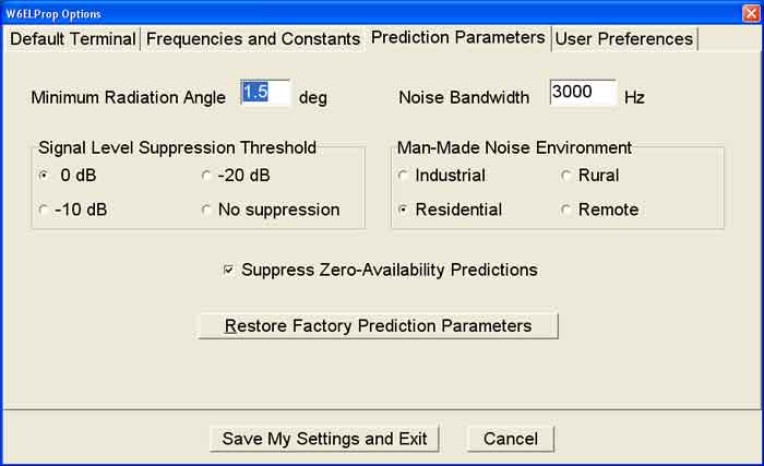
In next tab you’ll see “Predictions Parameters”. We will set here:
- Minimum Radiation Angle =1.5 If you live in an area where you have a mountain towards a direction you must increase this number
- Noise Bandwith =3000Hz For SSB predictions or 500Hz for CW predictions.
- Signal Level Suppression Threshold=0dB
- Man Made Noise Enviroment= Industrial or Rural or Residential or Remote. I have chosen Residential as I live in a city.
- Finally check Suppress Zero-Availability Predictions Box.
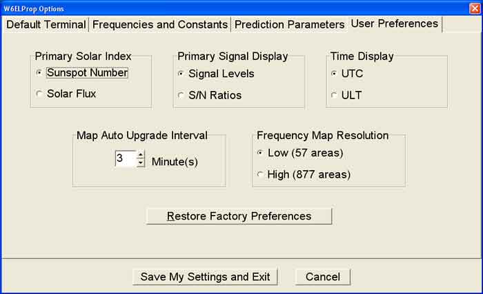
The last tab is “User Preferences”. We will set here:
- Primary Solar Index = Sunspot Number
- Primary Signal Display = Signals Levels
- Time Display = UTC
- Map Auto Upgrade Interval=3 minutes
- Frequency Map Resolution=Low or if you want higher map resolution choose High
Everyday use
After all of the above settings, don’t forget to click on “Save My Settings and Exit” to save all and exit from the options menu. You will return to the initial screen. We only needed to do all of the above once, as it was the first-run setup. After this it’s an easier task to make predictions. Choose “Predictions” in the menu and then “On Screen” to see predictions on your screen. Then you will see the next window.
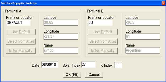
The callsign and geographical data are on left side under Terminal A. On the bottom left you’ll see Date. Here we must add the date we want predictions for. Let’s try a prediction for Argentina. If we know the prefix we add it. If not (shame on us) we can select it from Atlas where we can choose the Terminal B by name.
Do you remember that we had previously entered Primary Solar Index=Sunspot Number? So here we must add Sunspot number where it says Solar index. This number is the mean value of 13 months with the center on the desired date. That is 6.5 months before and 6.5 after the desired date. So you can understand that we don’t know this number. We must therefore use a prediction for the 6.5 months after.
One solution is to go to this page https://www.swpc.noaa.gov/products/predicted-sunspot-number-and-radio-flux and use the number in left column for let’s say “July 2019”. You can see year and month in left side and in column under Predicted as the number we need.
So from this table we can see that the predicted value for July 2019 for Solar Index is 2.1. Note also that there is a number called “Radio flux” also. If we have chosen “solar flux” for “Primary Solar Index”, this is what we must add (in our case is 69.3).
Why we must add the mean number of sunspots or solar flux? and not the daily number? Because the best approach for accuracy of our model is to compare mean values of solar and ionospheric data. So our prediction is statisticals.
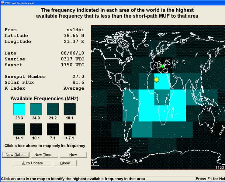
Put Κ =-1. This means that our predictions are for the mean value of K and click ΟΚ. After a few seconds you will see the next screen and on the bottom right you’ll see “click to see prediction”. In the same screen we can see prognosis data as geographical data of the two terminals, the sunrise and sunset time, Bearings and the distance for our signals (Short Path length and long path length). So click on Show Predictions and you will see the following picture .
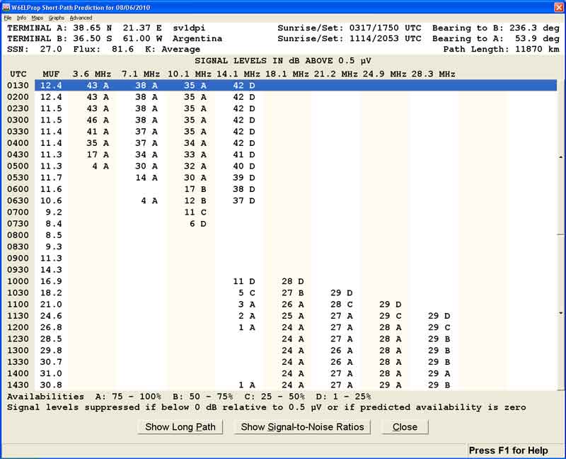
The first thing we can see is that there is a difference between low bands and high bands. When low bands have propagation, high bands don’t and vise-versa. Maybe we knew this already, without needing the program to tell us, as we have in mind that low bands are active during night and high bands are active during sunlight.
The first column is the time in UTC. The second column is the Maximum Usable Frequency where there is propagation between the two terminals.
We called it MUF.
Do you remember we said that our predictions are statisticals? That means that the predicted MUF is right for some days during the month but not for all. For example we know that at 1200 UTC, MUF will be 26,8MHz.
Does this mean that at 12:00 utc we can make a QSO on 12m between Greece and Argentina?
Yes and no. This is quite possible, but only for some days of the month and we don’t know which are these. Do we know at least how many days are the good ones? Yes, approximately. The letters A, B, C and D beside every number say the number of good days in every month. The software has 4 categories, and explains them at the bottom of the screen. For example in the previous prediction for 28.3 MHz at 1200UTC it displays C. This means that 10M will be open from Greece to Argentina from 8 to 16 days during June of 2010 (25-50%) at 1200 UTC. But as we saw before, we don’t know which are the good days. If we see at 1230 UTC, we ‘ll see that the probability increases to B (B=50-75%) that is from 16 to 24 days at 1230 UTC. So if we don’t have the time to be on the radio every day at every hour, it is better to be active at 12:30 compared to 12:00 in order to try a QSO with Argentina on 10M during June 2010.
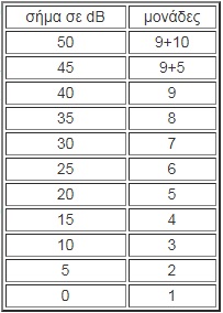
Now we know what the letter is. Let’s see what the number means. The number is the predicted signal in dB over 5μV. We know that S9 is 50μV and every S-unit is ~6dB (on newer rigs it’s significantly less). So the values in the program are translated according to the table of S-units. Don’t forget that we are talking about a mean value. So the actual signal might be a bit stronger or weaker. In the previous example, the signal will be around S7 (29dB).
This is the basic knowledge you need to work with the software. If you look into it deeper, you can see also find maps, MUF,etc. Good luck…