About Noise – plainly simple and easy to understand

About Noise

An attempt to describe, for fellow radio amateurs, the nature, types and characteristics of noise in a simple and understandable way, avoiding the use of mathematical relationships and formulas

Noise in telecommunication systems is defined as the sum of unwanted received frequencies on the one hand and those generated by the system stages on the other. It can be distinguished between fundamental noise and intermodulation noise.

Fundamental noise can be distinguished into exogenous noise (external), such as atmospheric, industrial, stellar, interference noise, and endogenous noise (internal), such as thermal, vacuum tube noise, semiconductor noise, power supply noise.

Intermodulation noise is mainly due to amplitude, frequency, or phase distortions, which are products of intermodulation.

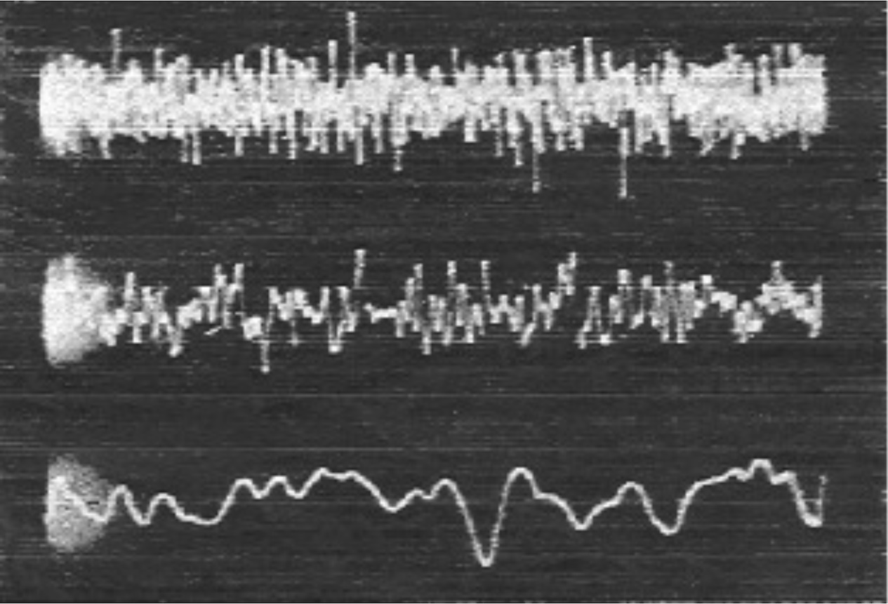
The main source of noise is the continuous and uninterrupted motion that characterizes nature on a microscopic scale. So, for example, in any piece of metal, we know that each molecule oscillates around its equilibrium position in the crystal lattice. And the conduction electrons of the metal move randomly within its free volume. The same happens with gas molecules that are confined within a space. These perturbations are called thermal perturbations because they increase with temperature. This random motion, mentioned above, gives rise to what is known as thermal noise (Johnson noise), which becomes zero at absolute zero (-273.15 °C or 0° K). This is why, for example, receivers in radio telescopes are cooled to cryogenic temperatures in order to minimize thermal noise as much as possible.

Another type of noise is that resulting from the flow of current through the contacts of semiconductors. Electrons or holes enter the contact area from one side ( P or N ), pass through the contact and are collected from the other side ( N or P ). The average value of the contact current is determined by the average time interval between the moments when the respective electric carriers (electrons or holes) enter the contact. However, this time duration is subject to some random ( statistical ) variation, which results in some noise called shot noise. Such noise also occurs during thermionic emission of electrons and therefore affects the devices that use this method (ie vacuum tubes).

When a signal arrives at the receiver it may be very weak so it needs amplification. This amplification is carried out by means of amplification circuits consisting of active and passive elements.

In line with what has been said above about these elements, it is logical that the amplification device will therefore also increase the noise level along with the signals that are amplified.

Especially in amplifiers that use vacuum tubes, apart from the aforementioned thermal noise, we can also distinguish the vacuum tube noise which occurs as a result of anomalies in the electron flow. This noise can be divided into the following categories:

Shot noise: occurs due to a change in the rate of thermionic electron emission from the cathode of the tube.

Partition noise: comes from the variations in flux as the electron beam diffuses through two or more electrodes in the vacuum tube.

Induced grid noise: This noise is caused by variations in the intensity of the current flowing through the grid of the vacuum tube.

Gas noise: This noise is produced due to disturbances in the rate of ion production from collisions.

Flicker noise: this noise results from low-frequency fluctuations during the thermionic emission of electrons from the oxide-coated cathode.

Noise due to secondary emission: This noise is produced due to secondary emission of electrons from the electrodes of the vacuum tube due to collisions with electrons heading towards the anode.
The noise that accompanies a signal can be either additive, i.e. added to the signal, or multiplied by the signal, so we are now referring to intermittent noise.

So we’ve touched briefly on the most common kinds of noise related to semiconductors and vacuum tubes, now let’s have a look at some other kinds of noise.

In the case of signal propagation in space (atmospheric or space), noise is introduced by the influence of celestial bodies (Sun, Moon, Stars, the Galaxy) and the atmosphere in the case of atmospheric propagation.

Atmospheric noise comes from sudden discharges of static electrical charges that accumulate in the atmosphere. These discharges generate current pulses with a duration of 0.1 μsec to 2 μsec and each such pulse generates a continuous frequency spectrum that occupies the entire radio wave range. Another cause of atmospheric noise is local storms.

Solar Noise : Noise that originates from the Sun is called solar noise. The intensity of solar noise varies over time in a solar cycle.

Cosmic noise: Distant stars generate noise called cosmic noise. While these stars are too far away to individually affect terrestrial communication systems, their large number leads to noticeable impacts. Cosmic noise has been observed in a range from 8 MHz to 1.43 GHz. Apart from man-made noise, it is the strongest noise component observed over the range of about 20 MHz to 120 MHz. Little cosmic noise below 20 MHz penetrates the ionosphere, while its eventual disappearance at frequencies in excess of 1.5 GHz is probably governed by the mechanisms generating it and its absorption by hydrogen in interstellar space.

If we summarize the above, we see that during the transmission of a signal a number of noises appear in it, both from the environment and from the device.

If we want to qualitatively compare two telecommunication systems taking into account the presence of noise, we need to know whether each of them is able to better separate the noise from the useful signal and thus rid it of distortion and errors.

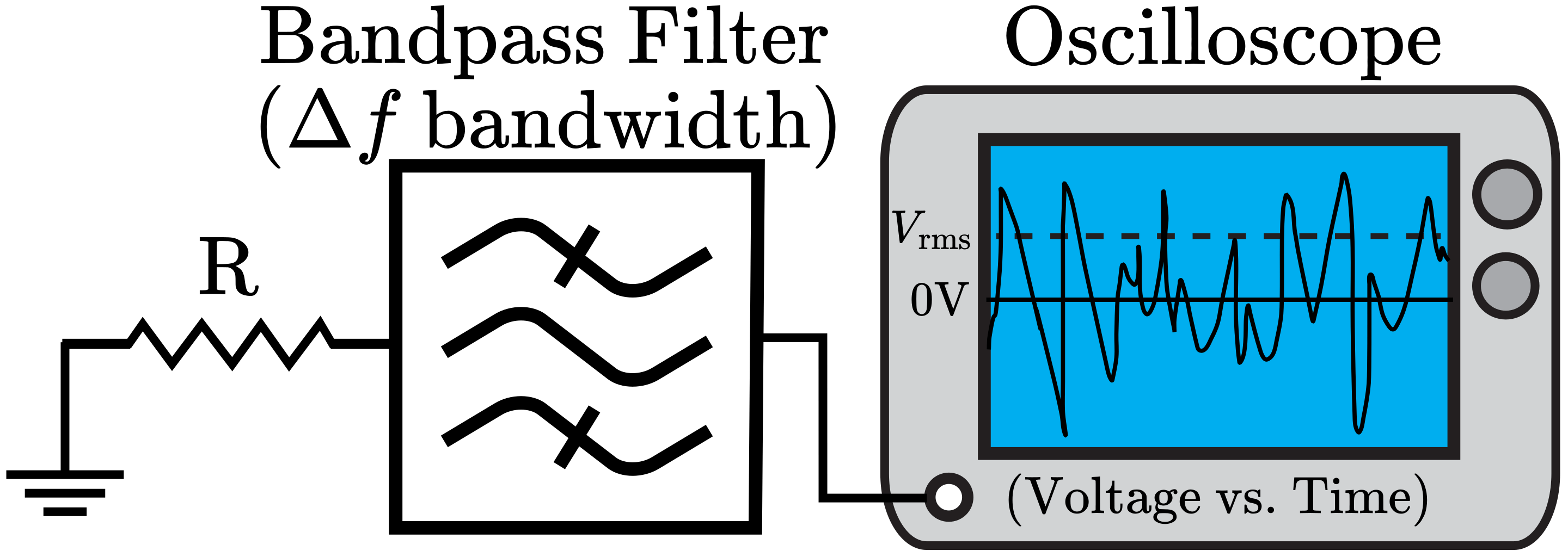
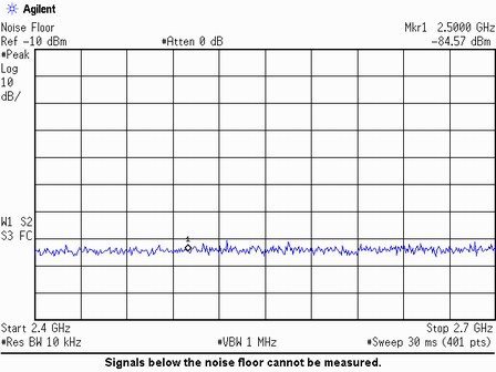
Noise can be quantitatively assessed by measuring with suitably calibrated instruments on a non-inductive resistance (resistive load) which terminates at the point on the device where we want to measure the noise. These instruments are voltage-measuring instruments that can be calibrated to give the signal or noise power value in dBm or mW.

Noise measuring instruments must have high sensitivity, very low internal noise and a uniform response curve for the frequency range in which we are interested in measuring the level. These instruments should measure the absolute value of the noise level.

The ratio of the noise power measured in a given frequency bandwidth, to that particular frequency bandwidth is called the noise power density.

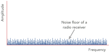
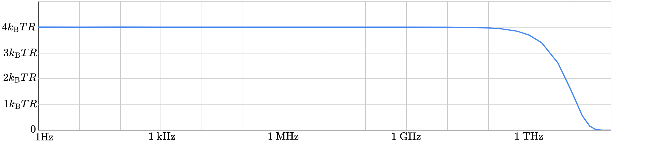
White noise: is a random signal having equal intensity at different frequencies, giving it a constant power spectral density.

Here we need to define some quantities the use of which will help us to calculate the noise figure of the receiver.

An interesting quantity is the insertion ratio, which is the ratio of the signal-to-noise ratio of the input to the signal-to-noise ratio of the receiver output: (S_in/N_in) / (S_out/N_out)

Available noise power: is that produced on a thermally excited resistor matched to a load and which at a specified temperature is equal to the power produced by the actual noise source on the load.

Noise temperature: at a given frequency is the temperature (in degrees Kelvin) of a passive element (or system of elements) with an available noise power per unit noise bandwidth equal to that of an actual noise source.

The noise presented at the input of our receiver is proportional to the bandwidth of the reception and is given by the relation n=kTB where k is Boltzmann’s constant, T is the temperature (Kelvin) and B is the reception bandwidth of our receiver. Therefore, to improve the S/N ratio at the input of our receiver we need to have a strong signal ( S ) and a small receiving bandwidth (narrow filter).

Noise Factor: The noise factor indicates the noise performance of the receiver. That is, how much noise the receiver adds to the noise it receives at its input. So by knowing the noise factor of a receiver we can estimate its quality in relation to its other characteristics such as sensitivity , selectivity etc.

Noise Figure: The noise figure is a measure of the degradation caused by the receiver components, it is the difference in decibels (dB) between the noise output of the actual receiver and the noise output of an “ideal” receiver with the same total gain and bandwidth. The lower the value of the Noise Figure, the better the performance of the receiver. The Noise Figure is the noise factor expressed in dB.

An Ideal Receiver is a receiver whose input has noise N_in = kTB and at the output N_out = G_gain kTB

According to the insertion ratio we have F = (S_in/N_in) / (S_out/N_out) = (S_in * N_out) / (S_out * N_in). (1) Because S_out/S_in = G_gain the inverse will be S_in/S_out = 1/G_gain so relation (1) becomes:

where F is the noise figure of the ideal receiver and G is the gain of the ideal receiver.

In a real receiver, we have the noise at the input N_in = kTB and at the output we have N_out = G_gain kTB or N_out = G_gain N_in + N_Rx (where N_Rx is the noise introduced by the receiver). According to the insertion ratio we have F = (S_in/N_in) / (S_out/N_out) = (S_inN_out) / (S_outN_in) (2) If we replace the numerator of relation (2) with its equal, we have F = (G_gainN_in+N_Rx) / (G_gainN_in) = (G_gainN_in) / (G_gainN_in) + (N_Rx / G_gainN_in) = 1 + N_Rx/G_gainN_in

Finally, the noise figure of the real receiver is:

This article aims to introduce us to the basic concepts that characterize noise. If we wanted to fully cover the topic of noise we would have to write much more, perhaps a book. However, let us confine ourselves to these few brief definitions, which may provide food for thought and the inspiration for us to research the fascinating subject of noise more.