

Smith Chart: The Ultimate Practical Guide for Radio Amateurs
The Smith Chart in practice: How to read the NanoVNA’s Smith Chart and make the right decisions about your antenna
Table of Contents
Acknowledgments and Credit
Acknowledgments and Credit: Special thanks to Konstantinos Panagiotopoulos, SV1AER, Electronics and Telecommunications Engineer and member of the Radio Amateur Association of Western Greece – SZ1A. Much of the material and technical explanations on which this practical guide is based come from his original writings, work, experience, and invaluable contributions.
PART 1: Understanding the Smith Chart
In this part, we will cover the basic concepts we need to read a Smith Chart correctly.
We will explore what impedance is, what R and jX mean, how they relate to resonance, SWR, and matching, and how all of this appears on the NanoVNA’s screen. The goal is not theory for its own sake, but to build the foundation we need to understand what our measurements are actually telling us.
What is the Smith Chart, and why was it created?
The Smith Chart takes its name from Phillip H. Smith, an American RF engineer who worked at Bell Labs in the 1930s. Smith developed the chart to simplify the tedious and complex mathematical calculations involved in impedance matching in transmission lines and antennas.
In 1939, Smith introduced the chart as a practical tool for solving a very real problem:
How can we quickly understand what is happening in a transmission line, meaning a cable or circuit that carries RF energy from the transmitter to the antenna, and how can we match the impedance correctly to transfer as much power as possible with as little reflection as possible?
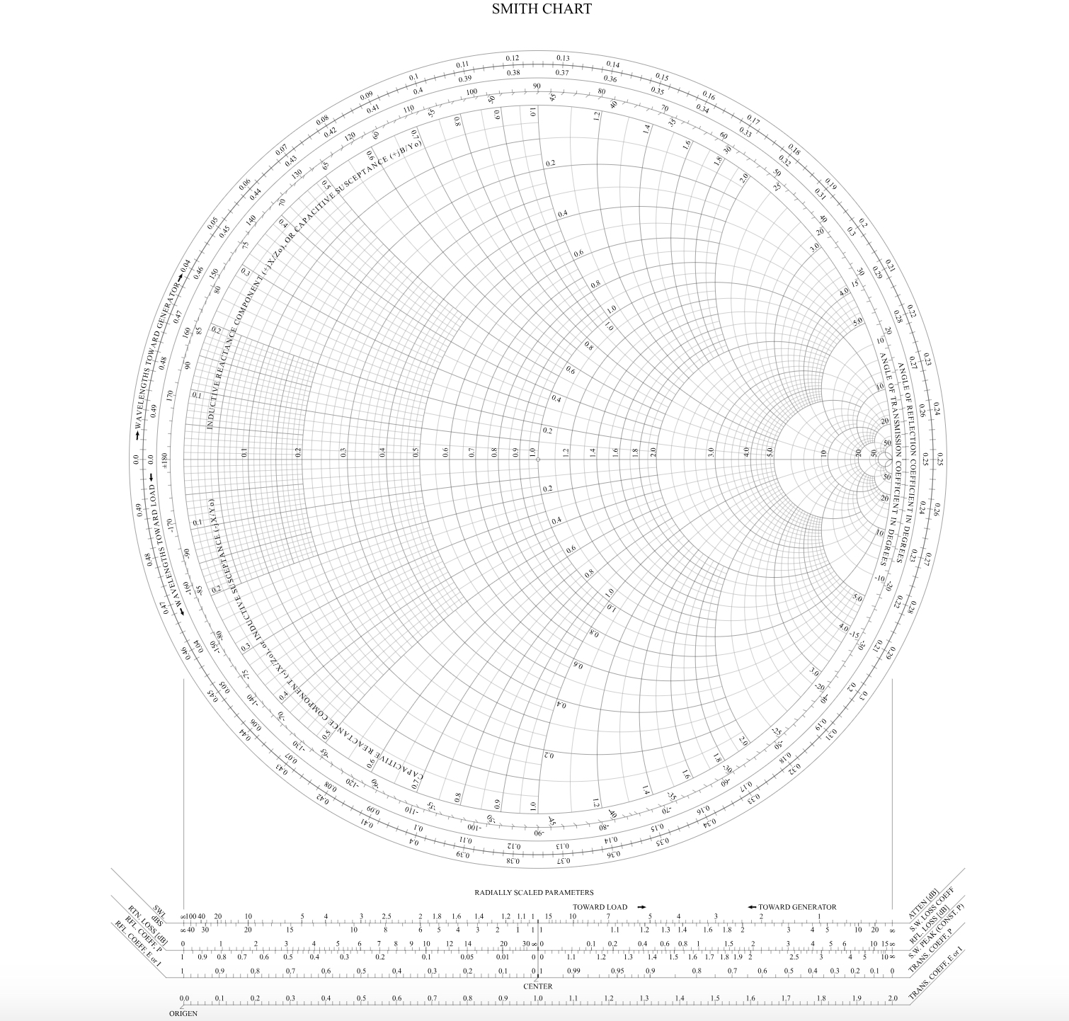
Throughout this article, we use technical terms such as impedance, reactance, complex number, reflection coefficient, characteristic impedance, and normalization. There is no need to be intimidated by them. We will explain each one as it comes up, focusing on its practical meaning rather than academic theory.
Before modern instruments such as the VNA became available, analyzing an antenna or a transmission line was a much more difficult process. RF engineers had to rely on complex numbers, transmission-line equations, and time-consuming calculations to understand what was actually happening in the system.
Originally, the Smith Chart was primarily a tool used on paper.
An engineer would take the necessary measurements or perform the calculations, then manually plot the impedance points on the chart to see how the load or transmission line behaved and determine the required matching. Modern VNAs have completely changed this process. They automatically measure the electrical behavior of a circuit at many frequencies and can display the results directly on a Smith Chart. What once required measurements, calculations, and plotting by hand now appears almost instantly as a trace on the instrument’s screen.
To understand why VNAs changed this process so dramatically, it is worth first explaining exactly what a VNA is.
VNA stands for Vector Network Analyzer.
In simple terms, it is an instrument that sends a known RF signal into an antenna, filter, coaxial cable, or other circuit, and measures what comes back and what passes through it.
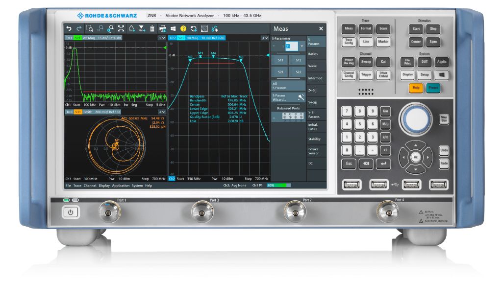
It does more than measure how much signal is lost or reflected. It also measures phase, meaning how the signal “rotates,” or shifts in phase, relative to the signal the instrument sent. This allows it to show us not only SWR, but also impedance, resonance, losses, the behavior of cables, filters, and baluns, and, of course, the Smith Chart.
For many decades, VNAs were expensive laboratory instruments. They were found mainly in professional RF, telecommunications, microwave, and industrial design laboratories. These were instruments for engineers, universities, and companies, beyond the reach of the average radio amateur. They could cost thousands or even tens of thousands of dollars, and using them required considerable technical knowledge.
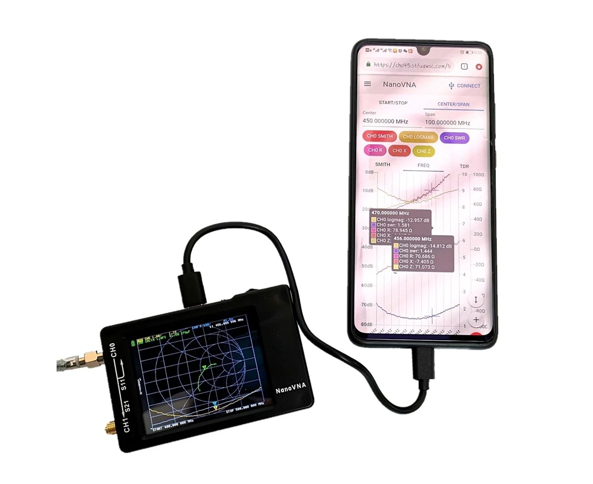
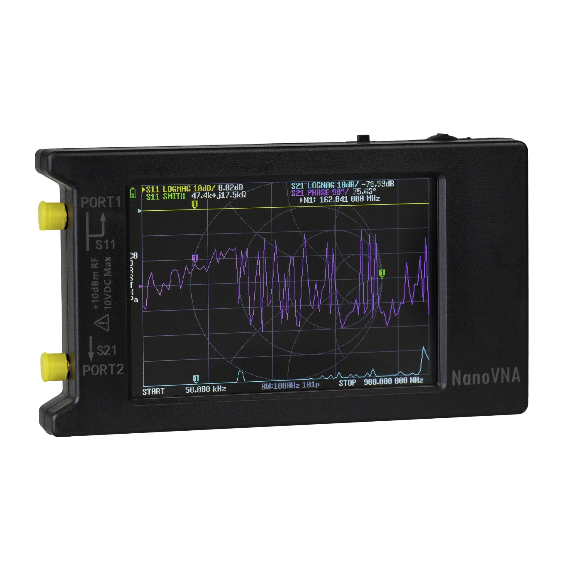
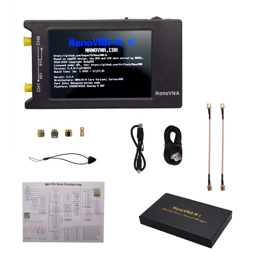
The big change came with the NanoVNA. Suddenly, a type of instrument that had once been prohibitively expensive for the average radio amateur became small, portable, and affordable. Often costing less than $50, depending on the version and where it is purchased, the NanoVNA gave radio amateurs access to measurements that had previously been confined to the laboratory.
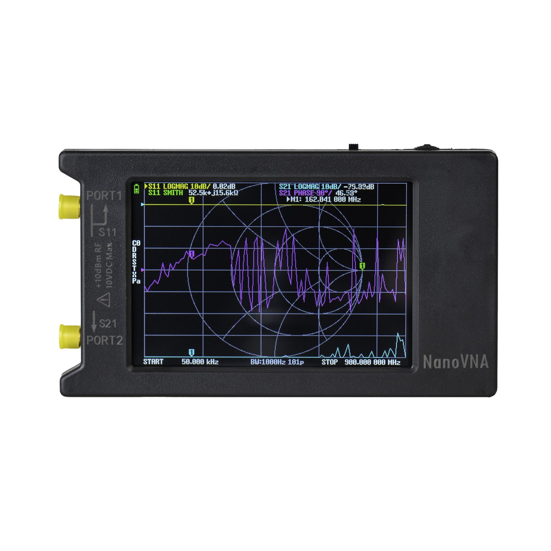
This is a real revolution for our hobby. We are no longer limited to looking at an SWR reading. We can see what is actually happening in the antenna, coaxial cable, balun, filter, or matching network.
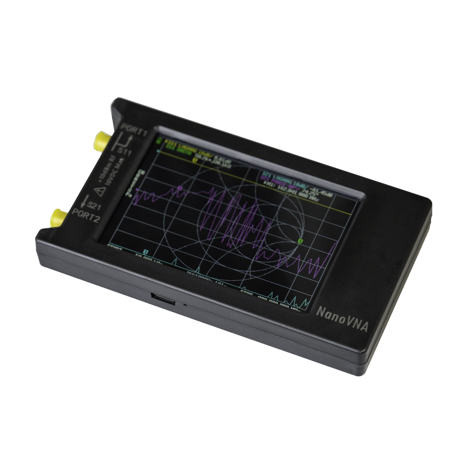
Let’s start with what really matters
The Smith Chart looks intimidating the first time we see it on a NanoVNA’s screen. It looks like a map filled with circles, curves, and strange points. And it is no coincidence that the Smith Chart has acquired an almost mythical reputation in the world of RF.
Many electrical engineering students describe it as “the scariest chart you encounter during your studies.” Professors often joke that it puts “the fear of God” into their students. Many compare it to looking into a vortex or a wormhole from a science fiction movie, while others jokingly call it “black magic and witchcraft.”
But there is a reason the chart has this unusual shape.
The Smith Chart achieves something that seems almost impossible at first glance: to “fit” even infinity inside a finite circle.
This very property is one of the things that allows it to represent the behavior of a transmission line or an RF load in such a practical way.
In practice, though, we do not need to become RF engineers to use it. We need to learn what the marker’s position means and what it tells us about the antenna, coaxial cable, tuner, and the point where we take the measurement.
This guide was written for Radio Amateurs. Not for exams in microwave theory.
The goal is simple: to be able to turn on the NanoVNA, look at the Smith Chart, and understand what our antenna needs.
When we measure an antenna with a NanoVNA, we usually want answers to practical questions:
- At what frequency does our antenna resonate?
- Is the antenna too short or too long for our intended frequency?
- Is the problem in the antenna, the coaxial cable, or the installation?
- Do we need to add or remove length?
- Are we dealing with common-mode currents, poor grounding, or unusual behavior caused by the surroundings?
- Is the tuner simply fooling the transmitter, or is it actually solving the problem?
The Smith Chart can help us answer all these questions because it reveals something that an SWR reading alone often hides.
SWR tells us how well or how poorly the system is matched, but it does not always tell us why.
The Smith Chart helps us understand the why as well, pointing us toward the source of the problem.
In our case, where the load is the antenna, we can determine whether it appears electrically short or long at the frequency we are interested in, and whether its resistance is lower or higher than the value we would like.
What is impedance?
In DC circuits, we usually talk about resistance. For example, a resistor might be 50 Ω. At RF, however, an antenna does not behave like a simple resistor. Its behavior changes with frequency and has two components: one that dissipates or radiates power, and one that temporarily stores energy and returns it.
Impedance (Z) is the overall “resistance” that an RF load presents to the signal. An RF load might be an antenna, a dummy load, or anything connected to the transmitter’s output. We call it impedance because, at RF, knowing how many ohms something has is not enough. We also want to know whether it behaves like an inductor or a capacitor. In antenna terminology, this is usually expressed as a complex number:
Z = R + jX
The term complex number sounds difficult, but here it means something simple: a number with two parts. The first part is ordinary resistance in ohms. The second indicates whether the antenna behaves like an inductor or a capacitor.
R is the resistance. It is the component associated with real power, whether that power is radiated by the antenna or lost as heat.
X is the reactance. It does not dissipate power like a resistor. Instead, it indicates that the load stores and returns energy, as inductors and capacitors do. The letter j is simply the mathematical notation we use to distinguish this “reactive” component from ordinary resistance.
- If X is positive, the behavior is inductive.
- If X is negative, the behavior is capacitive.
- If X is close to zero, the antenna is close to resonance at that frequency.
For radio amateurs, the practical point is this: we do not look only at SWR. We also look at jX, because it tells us which direction to take.
For example, with a simple half-wave dipole, measured at its feedpoint and near its resonant frequency, the practical rule is straightforward:
If jX is negative, the antenna usually needs to be lengthened.
If it is positive, the antenna usually needs to be shortened.
If jX is close to zero but R is not close to 50 Ω, the length may be correct, but impedance matching is needed.
In simple terms: impedance is the total opposition that an RF signal “sees.” It includes more than the ordinary resistance we know from Ohm’s law. At RF, we also care about whether the antenna behaves like an inductor or a capacitor. In other words, whether reactance is present alongside resistance.
This brings us back to the Smith Chart. The NanoVNA does the calculations for us, but the Smith Chart helps us understand what the measurements mean. It is not a decorative graph on the screen. It is a map showing how our antenna behaves, how its impedance changes with frequency, and how well it matches the standard 50 Ω system we use in transmitters, coaxial cables, and most measuring instruments.
We do not need to perform complex algebra to use the Smith Chart. We need to understand what R means, what jX means, and how they appear on the NanoVNA’s screen.
In simple terms, the Smith Chart helps us answer the question:
“What does our transmitter actually see when it looks toward the antenna?”
At this point, we need to clarify one more thing.
Throughout this article, we are talking about a typical 50 Ω amateur radio system.
This means we assume that the transmitter, coaxial cable, most measuring instruments, filters, dummy loads, and other station components use 50 Ω as their reference value.
However, this does not mean that the Smith Chart is inherently a “50 Ω chart.” The Smith Chart can be used with any reference value. This value is called the characteristic impedance or reference impedance, and we write it as:
Z0 = 50 Ω
In our examples, because we are discussing a 50 Ω amateur radio station, the center of the Smith Chart corresponds to:
Z = 50 + j0 Ω
That means 50 Ω of resistance and almost zero reactance. If we were working with a 75 Ω system, however, the center of the same Smith Chart would correspond to 75 Ω. So the chart itself is not “50 Ω.” The system determines which value we use as the center.
The Smith Chart at first glance
The first time we see a Smith Chart, it is natural to find it complicated. We see a large circle, lots of curves and numbers, and a trace or marker from the NanoVNA overlaid on all of them. But we do not need to understand every line right away.
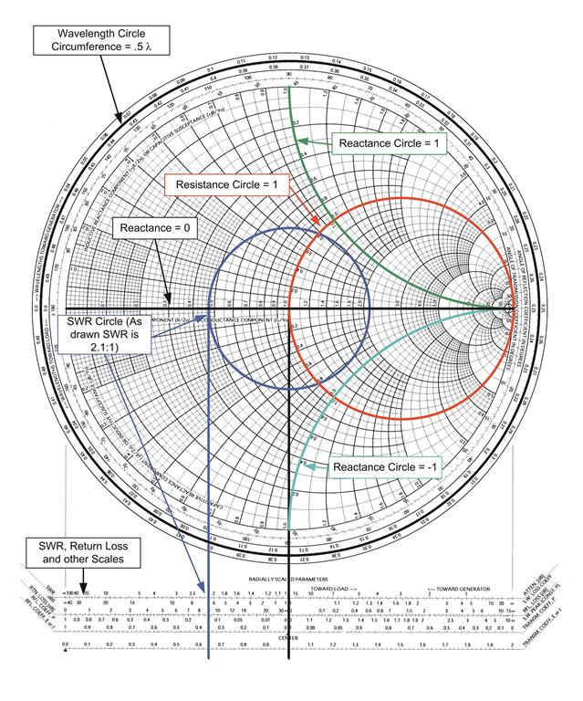
To begin with, it is enough to think of it as a map. The center is our reference point. The horizontal line through the center, or central horizontal axis, divides the circle into two halves: the upper half shows inductive behavior, and the lower half shows capacitive behavior. For points on the horizontal axis itself, resistance is lower than the reference value to the left of center and higher to the right. At the center, it is exactly equal to the reference value. In this article, because we are discussing a 50 Ω amateur radio system, that reference value is 50 Ω.
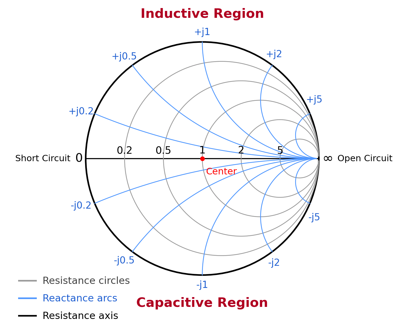
The many curves inside the chart are lines of constant resistance and constant reactance. We do not need to read every one individually to draw useful conclusions. At first, we are mainly interested in the general position of the point or trace shown by the NanoVNA.
For now, keep this basic picture in mind:
- Close to the center means a better match.
- Above the horizontal axis means inductive behavior.
- Below the horizontal axis means capacitive behavior.
- On the central horizontal axis, resistance is lower than the reference value to the left of the center, and higher to the right.
In the following sections, we will see what all of this means in practice and how to use it to make decisions about our antenna.
How to easily read a Smith Chart
Think of the Smith Chart as a map with four main regions.
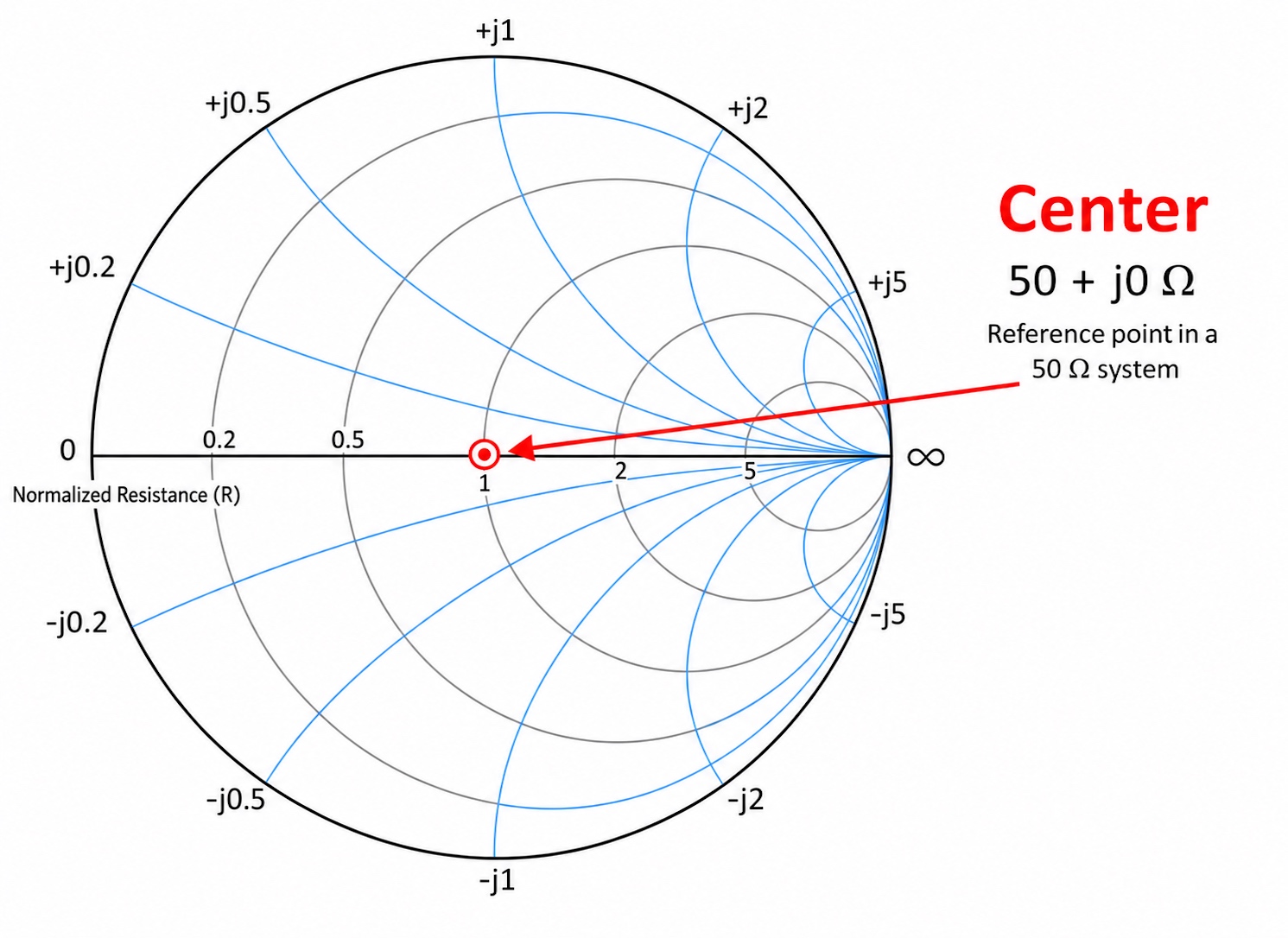
1. The center
The center represents the ideal match for a 50 Ω system. On the NanoVNA, we will see this as a reading close to 50 + j0 Ω.
If the marker is near the center at the frequency we are interested in, the antenna is close to a good match at that frequency. This is not the only thing we should look at, but it is a very useful first indication.
2. Above the horizontal axis
When the point is above the horizontal axis, the antenna appears inductive. This means we see positive jX on the NanoVNA. In practical terms, positive jX means the antenna behaves as though it has a small “inductor” inside it. For a simple center-fed antenna, this usually means it is electrically long for the frequency we are measuring.
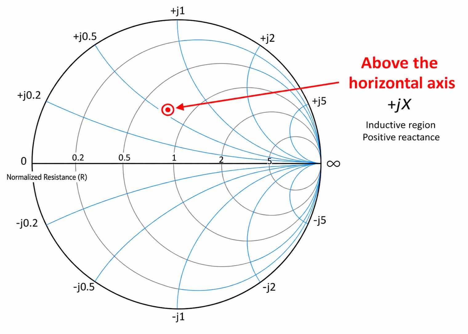
With a simple antenna such as a dipole, if we want to move its resonance higher in the band, we usually remove a little length.
3. Below the horizontal axis
When the point is below the horizontal axis, the antenna appears capacitive. This means we see negative jX on the NanoVNA. In practical terms, negative jX means the antenna behaves as though it has a small “capacitor” inside it. For a simple center-fed antenna, this usually means it is electrically short for the frequency we are measuring.
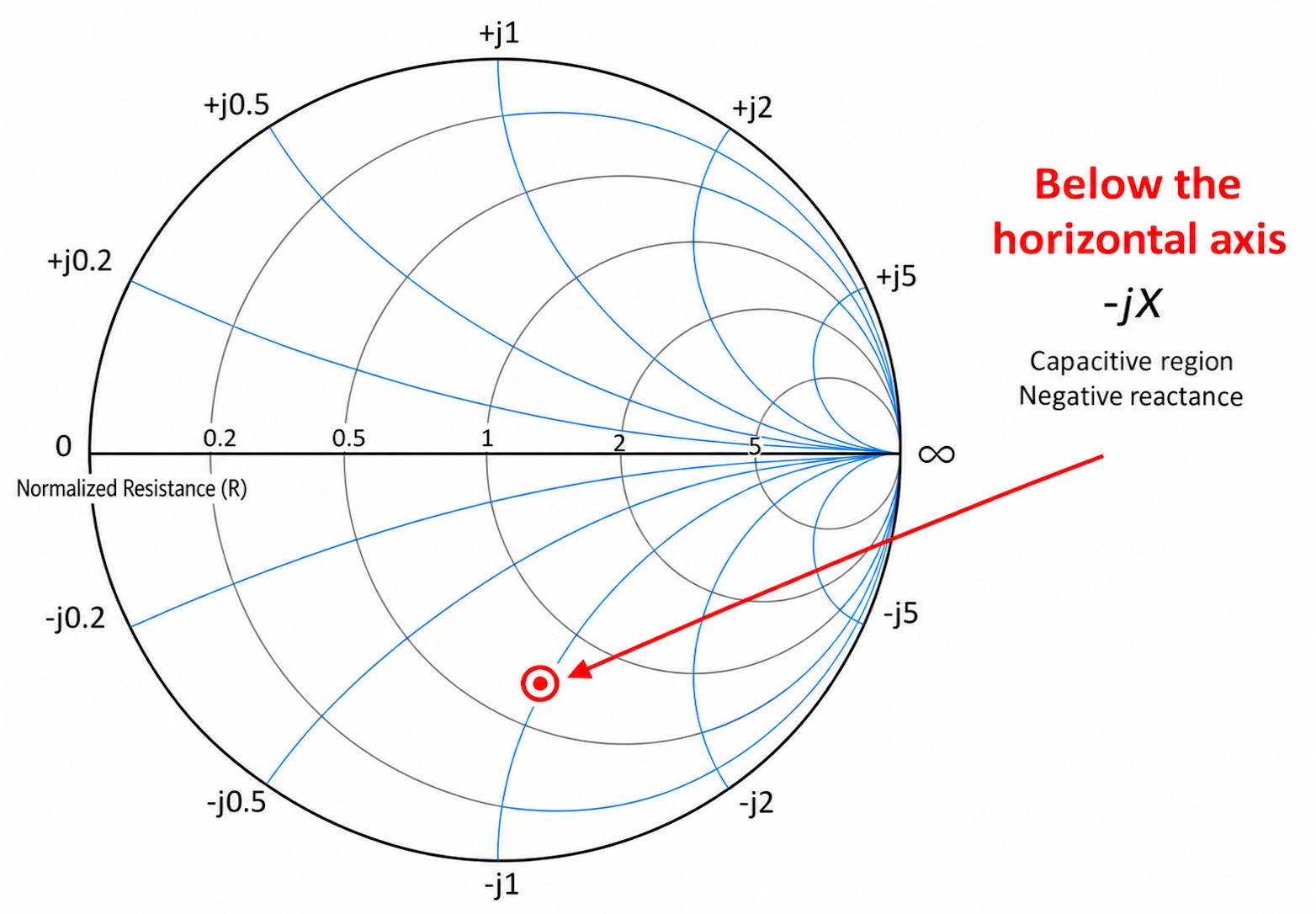
With a dipole, if we want to move its resonance lower in the band, we usually add a little length.
4. Left and right of the center
Here, we are looking at points on the central horizontal axis, where reactance is zero. Their position along the axis tells us the resistance, or the real part of the impedance. This is the component most similar to the resistance we know from basic electronics. In an antenna, however, it does not represent heat alone. It can also include radiation resistance, the component associated with power that is actually radiated as radio waves.
- Left of the center means the resistance is less than 50 Ω.
- Right of the center means the resistance is greater than 50 Ω.
- The far-left end of the horizontal axis theoretically corresponds to a short circuit, or 0 Ω.
- The far-right end of the horizontal axis theoretically corresponds to an open circuit, or infinite resistance.
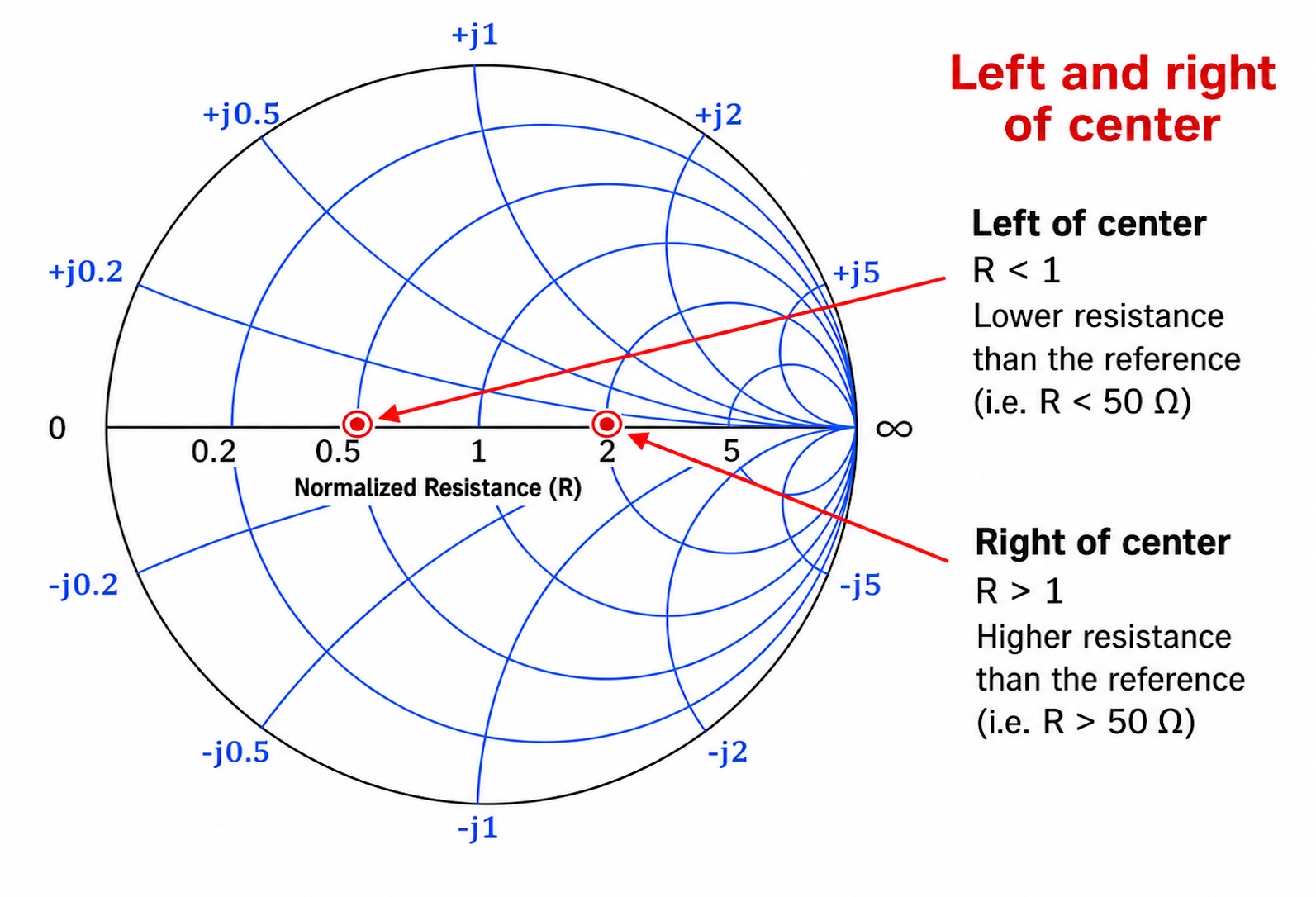
These endpoints are not where we want a normal antenna to appear. They are useful, however, for understanding what the chart is showing us when something goes badly wrong, such as a broken cable, a short circuit, or an antenna that is not connected properly.
The most important thing to remember about the Smith Chart
On the NanoVNA’s Smith Chart, the center represents a perfect match for a 50 Ω system. The impedance there is approximately 50 + j0 Ω, meaning about 50 Ω of resistance and nearly zero reactance.
Important: The center of the Smith Chart indicates both a good match and zero jX. However, a resonant antenna does not necessarily have an impedance of 50 Ω. Resonance means, first and foremost, that jX is close to zero. R can still have a value other than 50 Ω (for example, 200 Ω), and the antenna can be resonant but not matched to our 50 Ω system.
The closer the measured trace comes to the center, the better the match at that frequency. The farther the point is from the center, the greater the reflection and the higher the SWR tends to be.
There is more to reading the Smith Chart than judging how close a point is to the center. It also shows us whether the antenna is capacitive or inductive, whether its resistance is lower or higher than 50 Ω, and whether the trace has the shape we would expect. This helps us make practical decisions about whether to change the antenna’s length, check the coaxial cable, or use a matching network.
Normalization and reflection on the Smith Chart
The Smith Chart was designed to work with more than just one type of system, such as the 50 Ω systems we commonly use in amateur radio and other RF applications.
We can also use it with 75 Ω systems, such as those often used for television reception, as well as with systems that have other characteristic impedances.
What makes this possible is normalization.
In the field of RF and Smith Charts, normalization means that we do not look at impedance as an absolute value in ohms. We compare it with the characteristic impedance of the system, denoted by Z0.
In simple terms, we divide the impedance we measure by the characteristic impedance of the feedline.
z = Z / Z0
where:
Z is the actual impedance we measure.
Z0 is the characteristic impedance of the system, for example 50 Ω or 75 Ω.
z is the normalized impedance, meaning the impedance expressed as a ratio.
This way, the Smith Chart does not need to know whether we are working with a 50 Ω, 75 Ω, or 300 Ω system. All it sees is the relationship between the load impedance and the characteristic impedance of the line.
For example:
- In a 50 Ω system, a 50 Ω load gives: z = 50 / 50 = 1
- In a 75 Ω system, a 75 Ω load gives: z = 75 / 75 = 1
- In a 300 Ω system, a 300 Ω load gives: z = 300 / 300 = 1
In all three cases, the point lies at the center of the Smith Chart because the load matches the feedline.
This is why the center of the Smith Chart always corresponds to:
z = 1 + j0
which is equivalent to:
Z = Z0
In other words, the load impedance is equal to the characteristic impedance of the system, and there is no reactive component.
Normalization allows us to use the same Smith Chart for different systems without changing how we read it. Whether we are working with 50 Ω, 75 Ω, or any other characteristic impedance, the question remains the same:
“How well does the load match the feedline?”
Normalization helps us answer that question visually. It shows us where the load impedance falls on the Smith Chart, always in relation to the characteristic impedance of the transmission line.
When the point is at the center, the match is perfect. When it moves away from the center, the load no longer matches the line exactly.
When there is a mismatch between the load and the line, the load does not absorb all the RF energy. Some of that energy travels back toward the source.
This return of the signal is called reflection.
To describe how large the reflection is, we use a quantity called the reflection coefficient, denoted by the Greek letter Γ.
What is the reflection coefficient Γ, without getting lost in theory?
The reflection coefficient Γ tells us how much of the RF signal travels back toward the source when it reaches a load that does not match the line.
The symbol Γ is simply the Greek capital letter gamma. It is used internationally for the reflection coefficient.
In everyday practice, we do not need to calculate Γ by hand or even read it as a separate value on the screen.
The NanoVNA measures S11, which is essentially the reflection coefficient Γ, and uses that information to plot the trace on the Smith Chart and calculate values such as SWR.
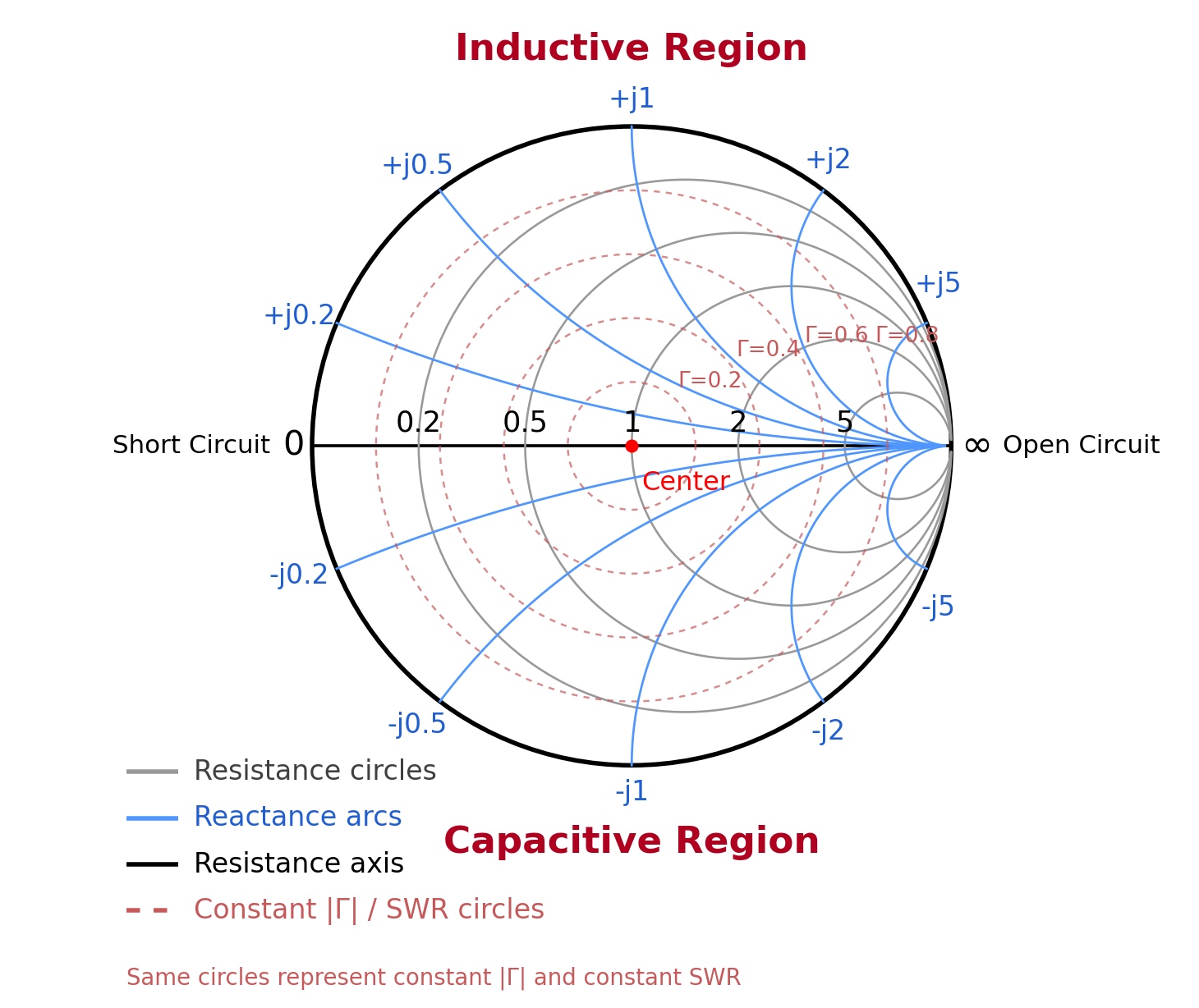
In practice:
- If Γ is zero, there is no reflection and the match is perfect.
- If the magnitude of Γ approaches 1, the reflection is very strong.
- On the Smith Chart, the distance from the center is related to the magnitude of the reflection.
- The farther the point is from the center, the higher the SWR reading.
If we want to keep just one picture in mind, it is this one. The center represents the best match, and the outer circle represents the worst. The farther the marker moves from the center, the greater the reflection.
To look at it a little more technically, we can define Γ from the relationship:
Γ = (ZL − Z0) / (ZL + Z0)
where ZL is the load impedance, for example, the impedance of an antenna, a filter, or any other device at the end of the transmission line. Z0 is the characteristic impedance of the transmission line. In most amateur radio RF systems, it is 50 Ω. In other systems, such as those used for television reception, it can be 75 Ω.
Γ is a complex quantity. It describes both the magnitude and the phase of the reflection. In practice, when we want to know how much reflection we have, we mainly look at |Γ|. This is the magnitude of Γ, also called its absolute value, and it is expressed as a real number.
On the Smith Chart, |Γ| corresponds to the distance of the point from the center:
|Γ| = 0 means no reflection. The load is perfectly matched to the line, and ZL = Z0 . This point is always right at the center of the Smith Chart.
0 < |Γ| < 1 means partial reflection. Part of the signal is delivered to the load, and part returns toward the source. On the Smith Chart, this corresponds to any point between the center and the outer perimeter.
|Γ| = 1 means total reflection. The entire signal returns, as it does in extreme cases such as a short circuit or an open-ended line. The point always lies on the outer perimeter of the chart.
In simple terms, the closer the measurement point (the marker) is to the center, the smaller the reflection. As the marker approaches the outer perimeter, the reflection becomes greater.
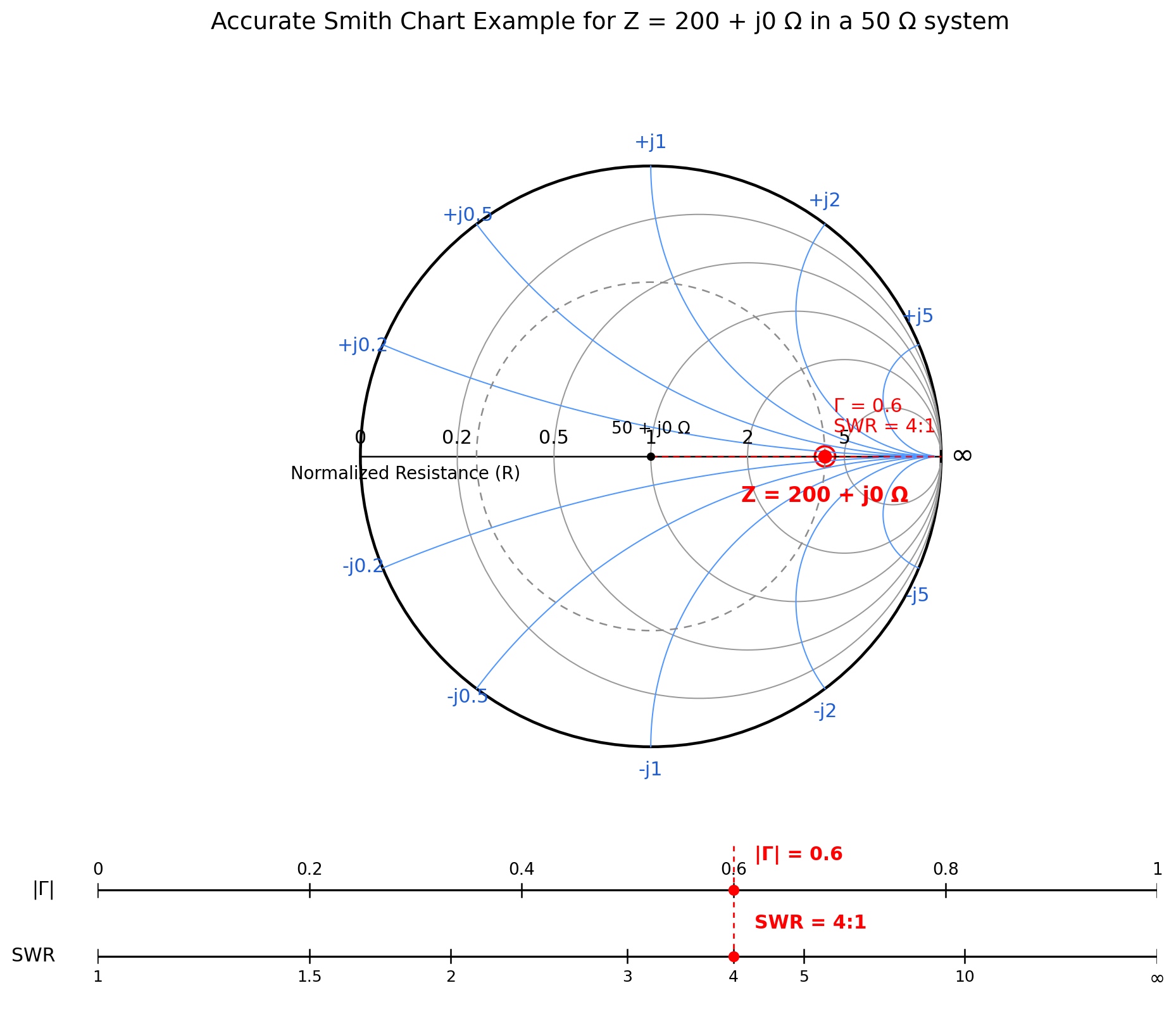
|Γ| is also directly related to SWR. The relationship is:
SWR = (1 + |Γ|) / (1 − |Γ|)
A few practical examples are all we need to see the relationship:
- |Γ| = 0 corresponds to an SWR of 1:1, a perfect match.
- |Γ| ≈ 0.33 corresponds to an SWR of about 2:1.
- |Γ| = 0.5 corresponds to an SWR of 3:1.
- |Γ| = 0.6 corresponds to an SWR of 4:1.
- |Γ| ≈ 0.82 corresponds to an SWR of about 10:1.
As |Γ| approaches 1, SWR rises very rapidly. When |Γ| = 1, we have total reflection, and SWR is theoretically infinite.
On paper Smith Charts and in teaching diagrams, this relationship is often shown on a ruler beneath the chart.
The upper scale shows |Γ|, and the lower scale shows the corresponding SWR. This lets us see immediately how a given reflection coefficient magnitude translates into SWR.
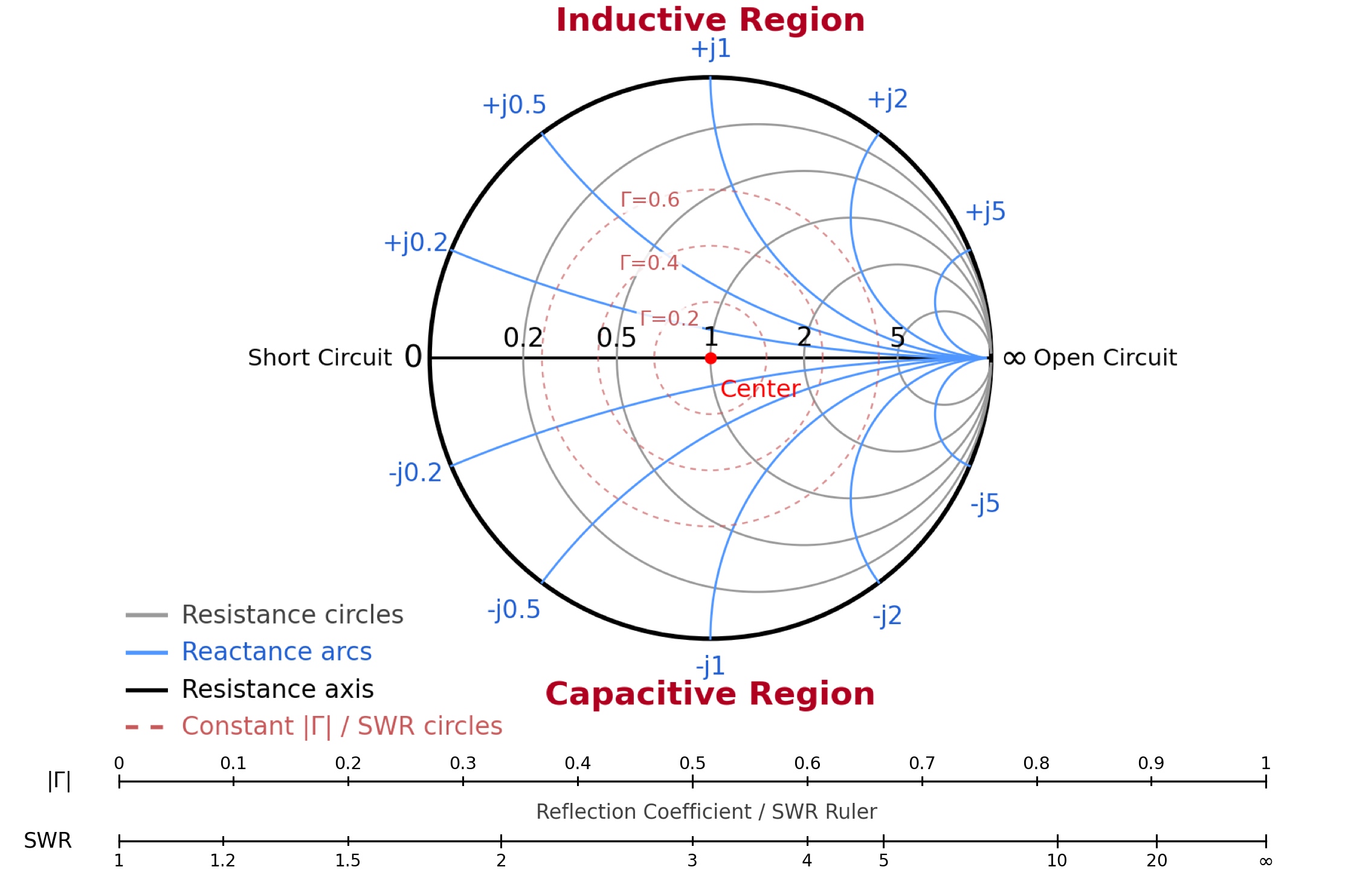
On a VNA such as the NanoVNA, the conversion is automatic. The instrument measures the reflection, calculates |Γ|, and displays the result directly as SWR on the screen.
For example, the NanoVNA can show the marker on the Smith Chart alongside a reading such as SWR 1.25 or SWR 2.10. The instrument has already converted the reflection coefficient information into a more familiar measurement value. We simply relate that SWR reading to the marker’s position on the Smith Chart.
Resonance and 50 Ω are not the same thing
This is one of the most important points in the entire article. Many radio amateurs confuse resonance with low SWR. They are not the same thing.
Resonance means that the reactance X is approximately zero. In other words, the antenna appears neither capacitive nor inductive at that frequency.
A good match in a 50 Ω system means that the impedance is close to 50 + j0 Ω. That means R is close to 50 Ω and X is close to zero.
An antenna can be resonant but not matched to 50 Ω.
For example, if the NanoVNA reads 200 + j0 Ω, then the antenna is resonant because jX is zero.
But in a 50 Ω system, we will see a high SWR because 200 Ω does not match 50 Ω.
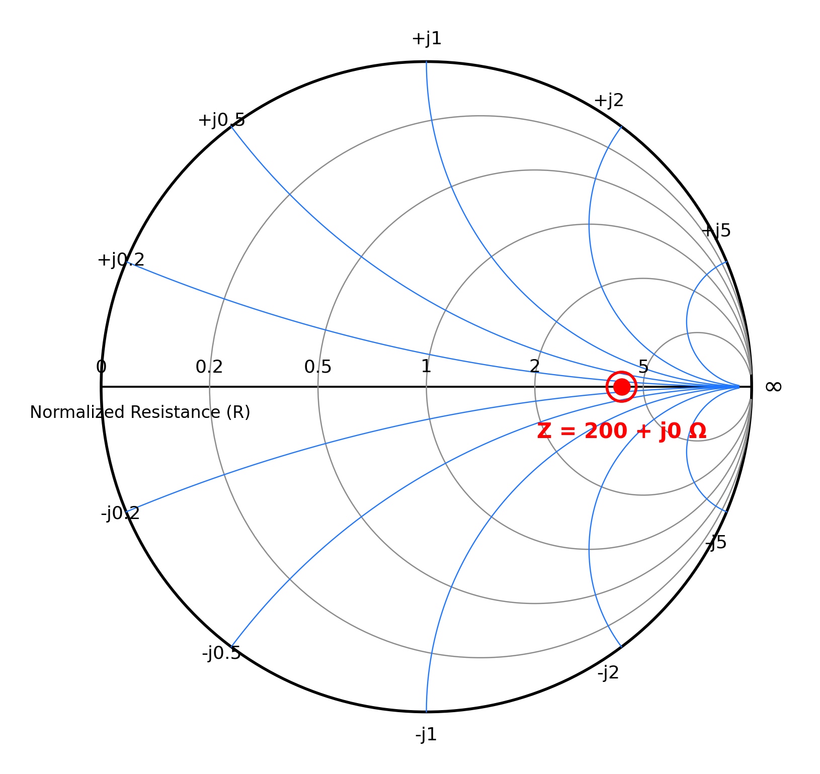
In this case, it would be wrong to simply say, “the antenna isn’t resonant.” It is. It just doesn’t directly match a 50 Ω line. Changing the length of the antenna is not necessarily the solution. The right solution may be a matching network or a suitable impedance transformer.
Example: If we have a balanced load of about 200 Ω and jX is close to zero, one practical solution might be a 4:1 current balun.
The 4:1 ratio transforms a load of about 200 Ω to about 50 Ω without changing the physical behavior of the antenna.
In other words, the antenna itself stays as it is, but the transmitter and the coaxial cable see a better-matched load.
The opposite can also happen. We can see a low SWR in the shack, either because we are using a tuner or because of losses in the coaxial cable itself, while the antenna remains strongly capacitive or inductive at its feedpoint. The transmitter may be “happy,” but that does not mean the antenna is actually resonant at the frequency we want.
PART 2: The Smith Chart in practice
This is where things get really useful.
We’ll see how to use the Smith Chart to tune an antenna, tell whether it is electrically short or long, and distinguish a resonance problem from a matching problem. We’ll also see how to identify common-mode currents and spot problems in the coax or at the feedpoint. All of this helps us make sound decisions before we start cutting, adding length, or changing things at random.
What the NanoVNA does when it displays the Smith Chart
When we sweep a range of frequencies, the NanoVNA measures impedance at many points within that range. To plot the impedance on the Smith Chart, it compares each measurement with the system’s reference impedance, usually 50 Ω. This comparison is called normalization. In simple terms, the instrument converts the values measured in ohms into a form that can be plotted on the same chart.
Each frequency corresponds to one point on the Smith Chart. Together, these points form a curve. The marker shows where one particular frequency lies on that curve. It is like a pin on a map. By moving the marker, we can see how our antenna behaves from the low end of the band to the high end.
This is much more useful than a single SWR reading because we can see how the antenna behaves across the entire sweep. We can see where it passes through resonance, where it becomes capacitive, where it becomes inductive, and how close its impedance comes to 50 Ω.
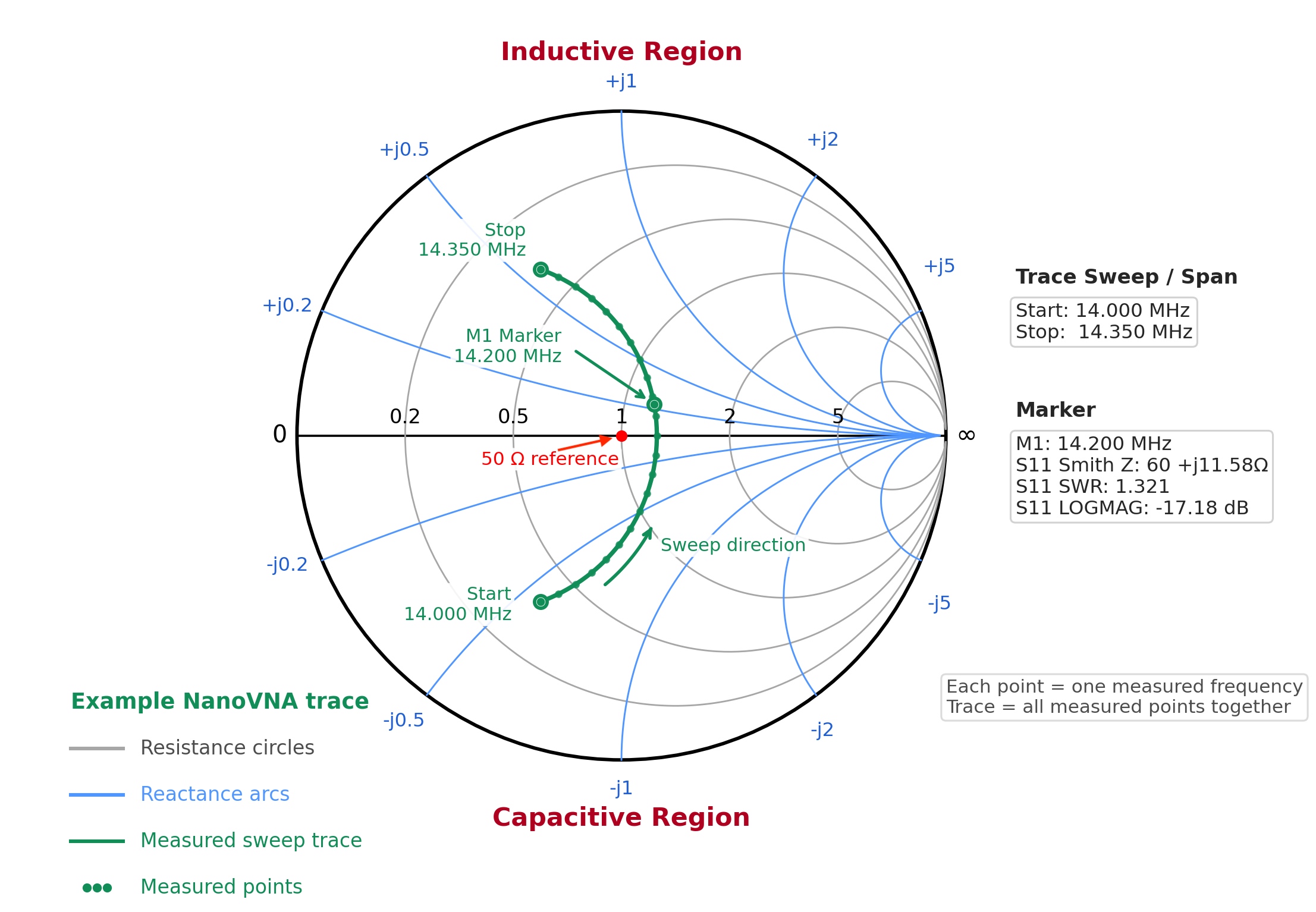
At the M1 marker in the example above, which corresponds to 14.200 MHz, we see that the antenna exhibits inductive behavior. We can tell because the marker lies above the horizontal axis of the Smith Chart, where jX is positive. For a simple center-fed antenna such as a dipole, this usually means it is slightly electrically long for that frequency.
At this point, the measured impedance is:
Z = 60 + j11.58 Ω
This value is not far from the ideal impedance our 50 Ω system would like to see:
Z = 50 + j0 Ω
Because of this, the resulting SWR is still quite acceptable:
SWR = 1.321:1
The curve, however, tells us something more useful than SWR alone. With a simple center-fed antenna such as a dipole, if we shorten it slightly to remove the inductive reactance, the trace will move toward the horizontal axis. Where the trace crosses the j0 line, the antenna is resonant because the reactance has reached zero.
The curve shows us which way we need to go. We make a small change in length and measure again to see the result.
In this example, that resonance point is approximately:
Z ≈ 62 + j0 Ω
This means we can bring the antenna into resonance by changing its length, but that adjustment alone will not bring its impedance to exactly 50 Ω. Even at resonance, the resistive part of the impedance remains about 62 Ω, not 50 Ω. There will still be a small mismatch in a 50 Ω system, with an SWR of approximately:
SWR ≈ 1.25:1
So, in practical terms, we can improve the match at 14.200 MHz by shortening the antenna slightly. This adjustment will remove most of the inductive reactance and bring the antenna closer to resonance.
The feedpoint impedance, however, will remain at about 62 Ω, so there will still be a small mismatch. In other words, with this antenna as it is, changing its length alone will not give us a perfect 1:1 match.
That is the beauty of the Smith Chart. We can see this before we make any physical change to the antenna. With an antenna analyzer that displays only numerical values for impedance and reactance, this might not be obvious. We might think that all we need to do for a perfect match is bring the reactance to zero. As this example shows, that is not the case.
The trace on the Smith Chart shows us what will actually happen if we change the length of the antenna. It shows us that shortening the antenna will remove the inductive reactance and bring it into resonance, but the feedpoint resistance will remain at about 62 Ω, not 50 Ω. The antenna will therefore be resonant, but it will still fall short of a perfect match to the 50 Ω feed line.
If we wanted a better match to 50 Ω, we would need to add a matching network at the antenna feedpoint. We could use an LC network, an impedance transformer, or another suitable matching method. This network would transform the antenna’s feedpoint impedance from approximately:
ZL ≈ 62 + j0 Ω
to the system impedance:
Z0 = 50 Ω
The transmission line would then see a much better match to 50 Ω, while the antenna would remain resonant.
This is why the Smith Chart becomes more useful than a simple antenna analyzer reading. A simple impedance and SWR reading tells us what is happening at one particular frequency, but the trace on the Smith Chart shows us the direction of the change. It helps us see where the point will move if we shorten or lengthen the antenna.
In this example, the trace shows that shortening the antenna will cancel the inductive reactance and bring it into resonance, but it will not bring the feedpoint impedance exactly to 50 Ω. That means we can avoid the common mistake of cutting or adjusting the antenna again and again, expecting a perfect 1:1 SWR that this particular antenna cannot achieve by length adjustment alone.
Practical procedure for NanoVNA measurements
To use the Smith Chart correctly, we follow a simple procedure.
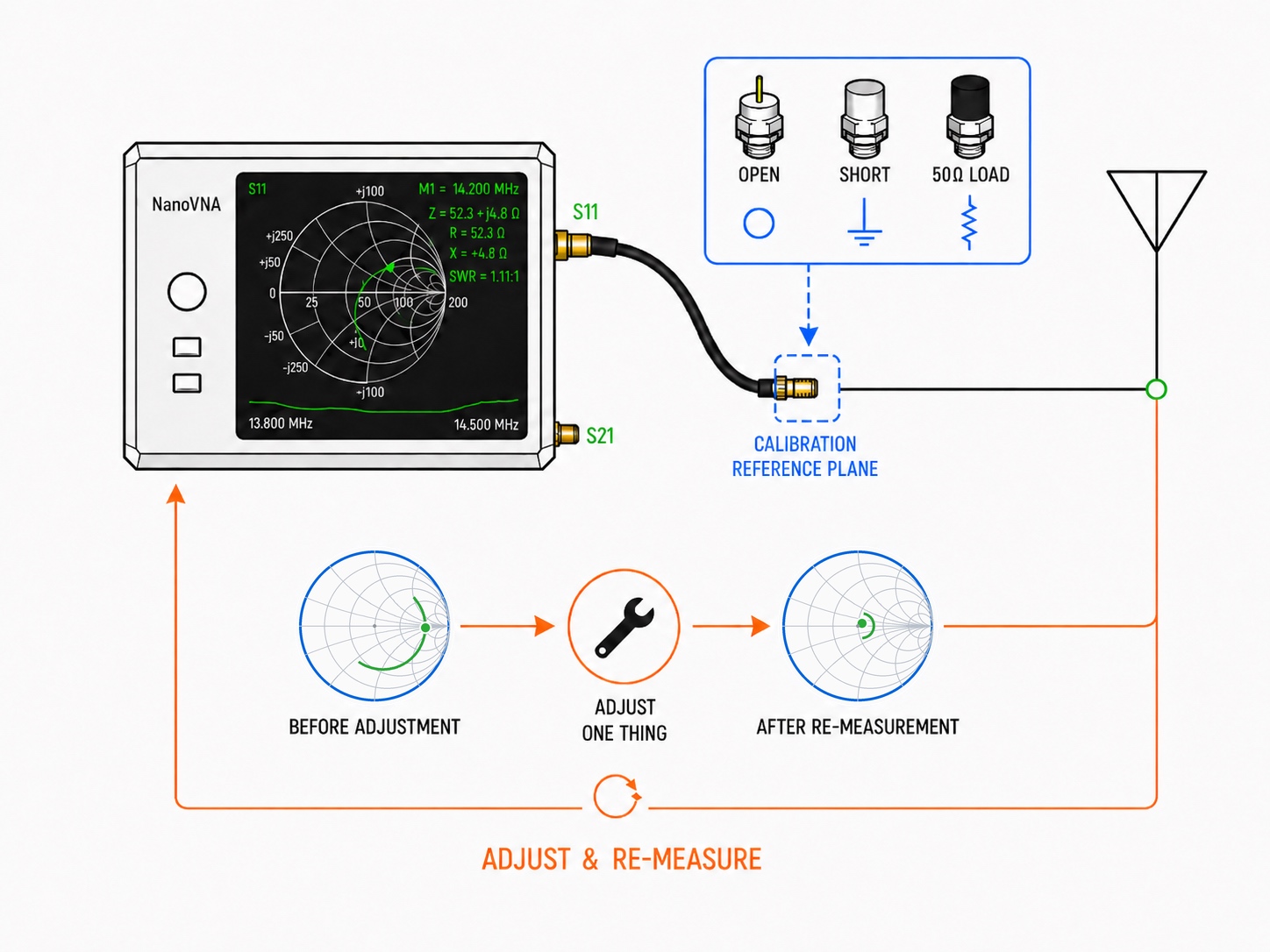
- We calibrate the NanoVNA over the frequency range we are interested in and at the point where we will take the measurement. If we use a test cable or an adapter, we calibrate at the far end of that cable or adapter. During calibration, we show the NanoVNA what a known open, short, and load look like so it can correct for the errors that the cable and adapters introduce into the measurement.
- We use the proper open, short, and load calibration standards. Open means an open circuit, short means a short circuit, and load means a proper 50 Ω reference load.
- Whenever possible, we measure as close as we can to the antenna feedpoint. If we measure from the shack through the feed line, we need to remember that we are seeing the antenna together with the transmission line.
- We set a reasonable frequency span around the band we are interested in. For example, on 20 meters, we might sweep from about 13.800 MHz to 14.500 MHz.
- We place the marker at the frequency we are actually interested in, rather than simply placing it where the SWR appears lowest.
- We look at jX first. If it is positive, the system we are measuring appears inductive. If it is negative, the system appears capacitive. These readings help us understand how our system behaves. For example, suppose we measure a simple half-wave dipole at its feedpoint, near its resonant frequency. An inductive reading usually means the dipole is electrically long for the frequency we are interested in and we need to shorten it slightly. A capacitive reading usually means it is electrically short and we need to lengthen it slightly. If jX is close to zero, we are close to resonance at that particular measurement point.
- Next, we look at R. If jX is close to zero, we are close to resonance at that particular measurement point. If R is well below or well above 50 Ω, however, the antenna can be resonant but still be poorly matched to our 50 Ω system. In that case, we need to look beyond simply changing the antenna’s dimensions. We need a way to match or transform the impedance, using a device such as an unun, balun, transmatch, or transformer, so the load is a better match for the transmission line and the transmitter.
- We look at the shape of the trace on the Smith Chart. If the trace is unstable, has an unusual shape, or changes when we move the feed line, we check the installation, the cables, the balun or unun, and the choke. We also check for common-mode current.
- We make one change at a time and measure again. If we change the antenna length, the balun or unun, the radials, the counterpoise, and the routing of the feed line all at once, we have no way of knowing which change affected the result.
What a “good” trace looks like
There’s no single perfect trace for every antenna. A dipole, a vertical, a loop, and an end-fed antenna all behave a little differently. What we want is a trace that makes sense, stays stable, and looks the way we’d expect for the type of antenna we’re measuring.
- The trace should be relatively smooth across the band we’re measuring.
- For a simple antenna, such as a center-fed half-wave dipole, the trace should move from capacitive to inductive behavior as the frequency increases.
- The point where jX reaches zero indicates electrical resonance.
- The point where R is close to 50 Ω and jX is close to zero indicates a good match to a 50 Ω system.
- The trace shouldn’t shift dramatically when we touch the cable or move the feed line slightly.
- Odd loops, sudden jumps, and an unstable reading tell us that something else is affecting the measurement.
If we see something unexpected, we don’t immediately start trimming the antenna. First, we check the connectors, coax, balun, grounding, and radials, and look for common-mode current.
What we see in this example
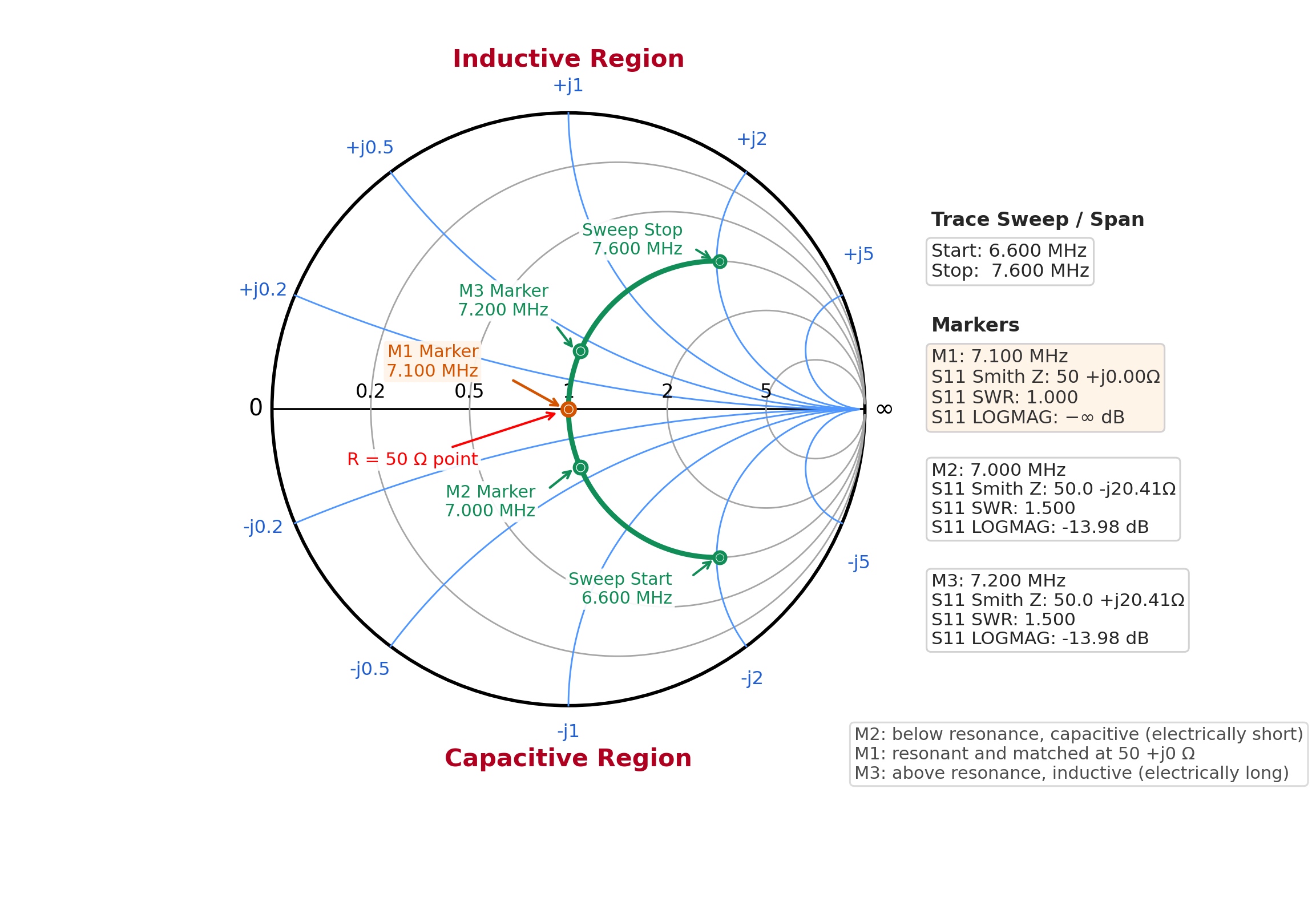
In this example, a 40-meter band antenna gives us a smooth trace with the shape we’d expect. The sweep starts at 6.600 MHz and stops at 7.600 MHz, so we can see how the antenna behaves both within the band and at frequencies below and above it.
The most important point is marker M1 at 7.100 MHz, right in the middle of the 40-meter band. At that frequency, the trace passes through the exact center of the Smith Chart:
Z = 50 + j0 Ω
SWR = 1.0:1
This means that, at this frequency, the antenna is both resonant and perfectly matched to a 50 Ω system. The reactance is zero, so the antenna is neither capacitive nor inductive. At the same time, the resistance is 50 Ω, exactly what the transmitter and feed line want to see.
At marker M2 at 7.000 MHz, which is at the lower edge of the band, the point lies below the horizontal axis. This indicates capacitive behavior, just as we’d expect for a dipole since we’re below the resonant frequency and the antenna is electrically short. Here, the measurement is:
Z = 50 − j20.41 Ω
SWR = 1.5:1
At marker M3 at 7.200 MHz, which is at the upper edge of the band, the point lies above the horizontal axis. This indicates inductive behavior, again just as we’d expect for a dipole since we’re above the resonant frequency and the antenna is electrically long. Now, the measurement is:
Z = 50 + j20.41 Ω
SWR = 1.5:1
This is a good example of a trace because the transition is smooth and follows the pattern we’d expect. As the frequency increases, the antenna starts out capacitive, reaches resonance at j0, and then becomes inductive. We don’t see any sudden jumps, odd loops, or unstable behavior.
We can also see something important. Within the 40-meter band itself, from 7.000 to 7.200 MHz, the antenna stays very well matched. At the center of the band, the SWR is 1:1, and at either end it’s still only about 1.5:1. This tells us the antenna performs well across the entire usable portion of the band.
The value of the Smith Chart here is that it shows us more than three individual SWR readings. We can see how the antenna behaves throughout the sweep. We can see whether the trace is smooth, whether it passes through the right point, whether the antenna is capacitive below resonance and inductive above it, and whether its behavior is what we’d expect from a simple dipole antenna.
Put simply, this is what we want to see in a “good” trace. It should be stable, smooth, predictable, and close to the center of the Smith Chart across the band we’re interested in.
Practical example 1: Tuning a Dipole for 20 meters
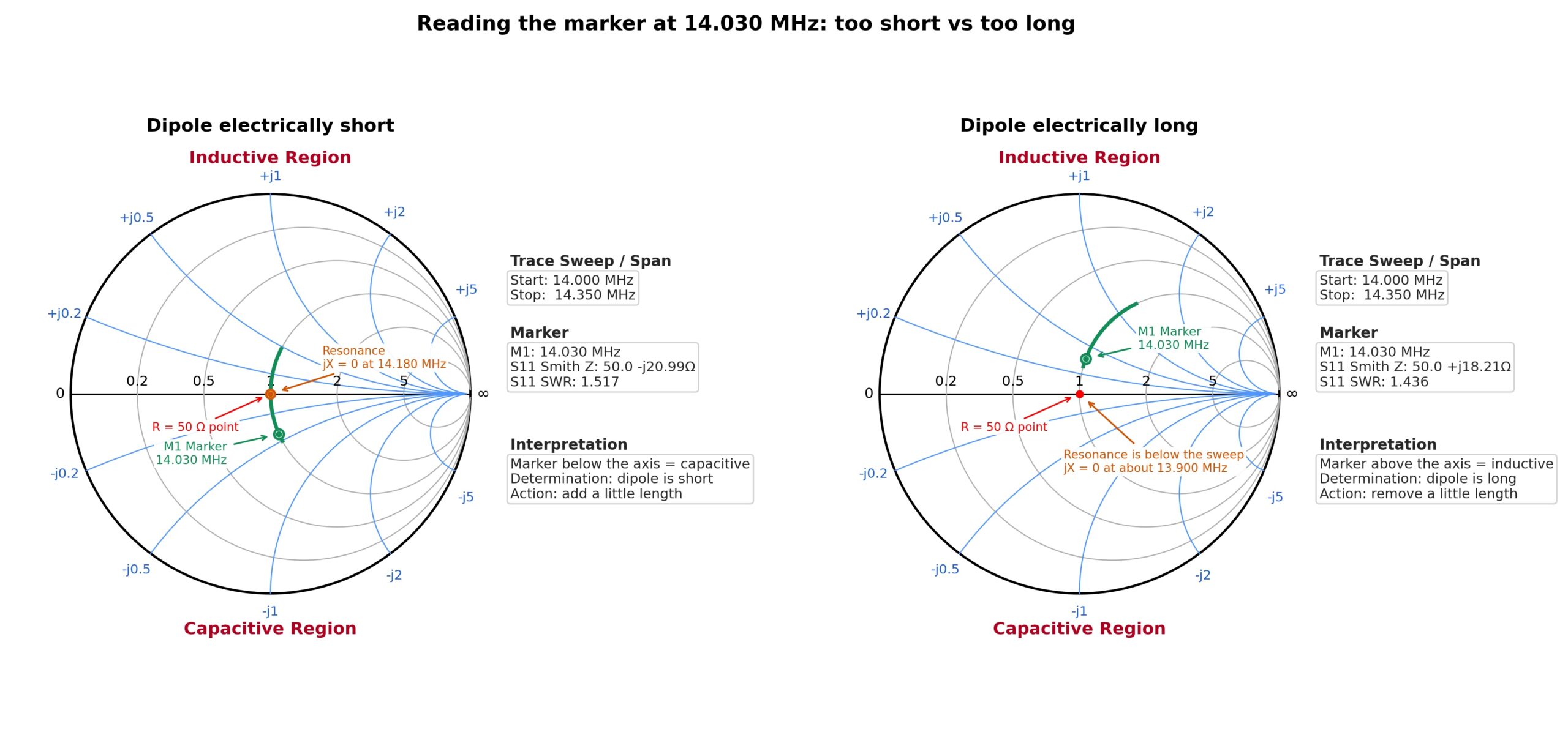
Let’s say we have a 20-meter dipole and want to use it mainly for CW near 14.030 MHz. We set the NanoVNA to sweep from about 14.000 MHz to 14.350 MHz and look at the Smith Chart.
We place a marker at 14.030 MHz and look at two things, first jX and then R. The jX reading tells us whether the dipole is electrically short or long at that frequency. R tells us how close the antenna’s resistance (the resistive part of its impedance) is to 50 Ω. In simple terms, it tells us how close the antenna is to the match we want in a 50 Ω system.
What we see on the Smith Chart
- If the marker at 14.030 MHz is below the horizontal axis, jX is negative. The dipole is electrically short at that frequency.
- If the trace approaches the horizontal axis as we increase the frequency and crosses it at 14.180 MHz, then the dipole’s electrical resonance is at about 14.180 MHz.
- If we want resonance at 14.030 MHz, the antenna is resonating too high. That means it’s short for the frequency we’re interested in.
What should we do next
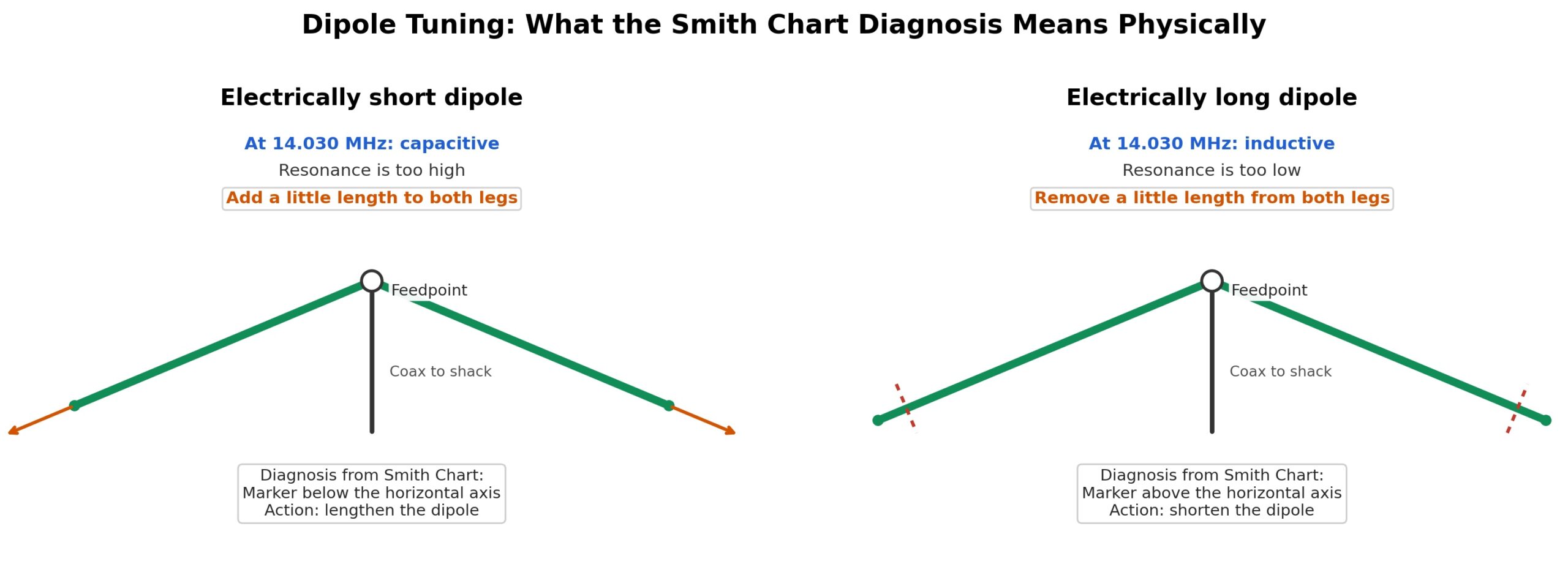
- Add a little length to both legs of the dipole.
- Measure again over the same frequency span.
- Check whether the point where jX is close to zero has moved toward 14.030 MHz.
- Repeat the process in small steps. Don’t trim or add too much wire at once.
If we see the opposite, with the marker above the horizontal axis at 14.030 MHz and jX positive, the dipole is electrically long. In that case, we trim a little off and measure again.
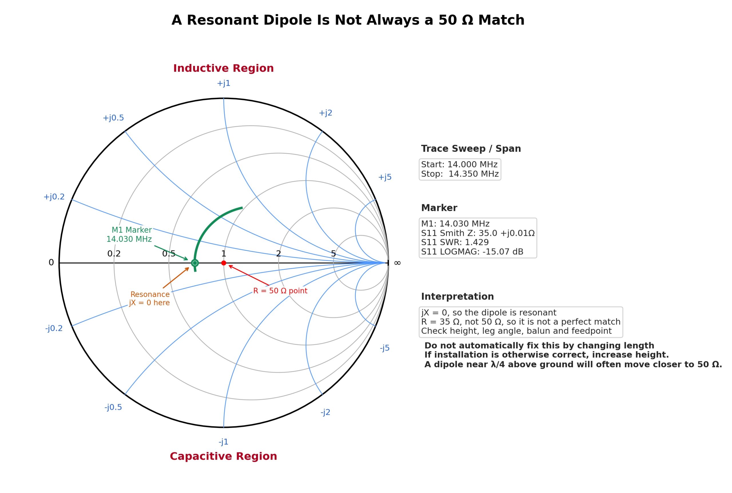
Important: If jX is zero but R is, for example, 65 Ω or 35 Ω, the dipole can be resonant without being perfectly matched to 50 Ω. Changing its length isn’t necessarily the way to correct the mismatch. First, we check the installation, the height of the dipole, the angle between its legs, the balun, and the feedpoint.
Practical example 2: A 1/4 λ Vertical Antenna with low resistance
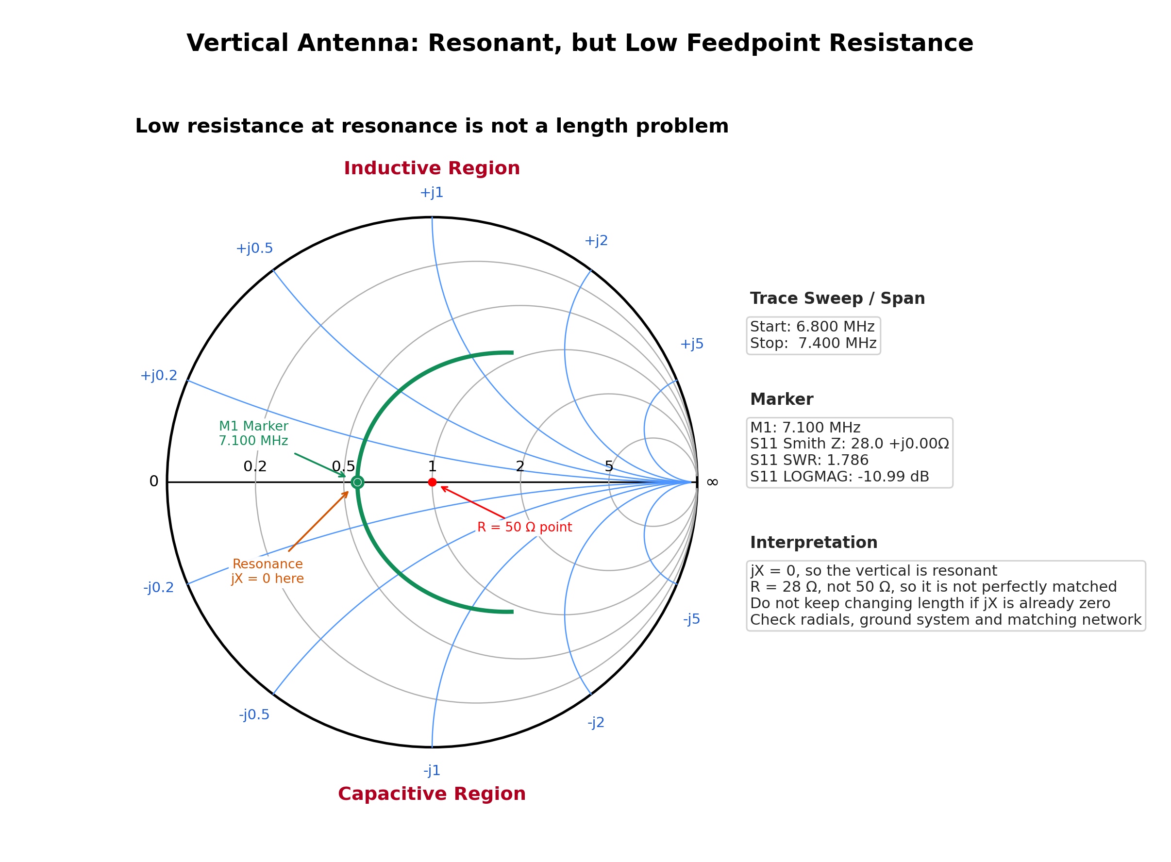
With a 1/4 λ vertical antenna that has radials, we may see the trace pass close to the horizontal axis but to the left of center. For example, the marker at the frequency we’re interested in might read about 28 + j0 Ω.
What this means
The jX reading is close to zero, so the antenna is close to resonance. It appears neither capacitive nor inductive. But R is 28 Ω, not 50 Ω. That is why the SWR in a 50 Ω system will not be ideal.
This doesn’t necessarily mean we’ve cut the antenna to the wrong length. Many verticals have a lower feedpoint resistance, depending on the ground, the antenna height, the radials and their slope, and the losses in the system.
How can we tell the difference on the Smith Chart
- If the point is on the horizontal axis but to the left of center, the issue is mainly one of resistance matching, not resonance.
- If the point is below the axis, the vertical is electrically short. Depending on the antenna, we may need to lengthen it or add inductive loading.
- If the point is above the axis, the vertical is electrically long. It usually needs to be shortened or adjusted in some other way.
What should we do next
- If jX isn’t zero, we first adjust the length or the loading so that the point falls on the horizontal axis at the frequency we want.
- If jX is zero but R is low, we don’t keep trimming or lengthening the antenna for no reason.
- Check and improve the radials because they affect both the antenna’s efficiency and its feedpoint resistance.
- If the antenna remains resonant but R is still below 50 Ω, we use a suitable matching network at the feedpoint.
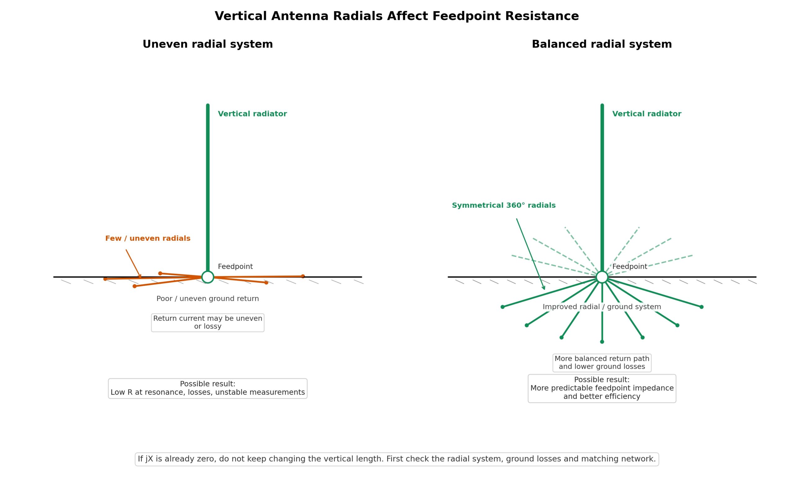
Conclusion: In simple terms, a reading of 28 + j0 Ω doesn’t mean the antenna is off resonance. It tells us the antenna is resonant, but isn’t matched to 50 Ω. So we treat this as a resistance matching issue rather than a question of antenna length.
Practical example 3: Low SWR in the shack, but the Smith Chart shows a problem
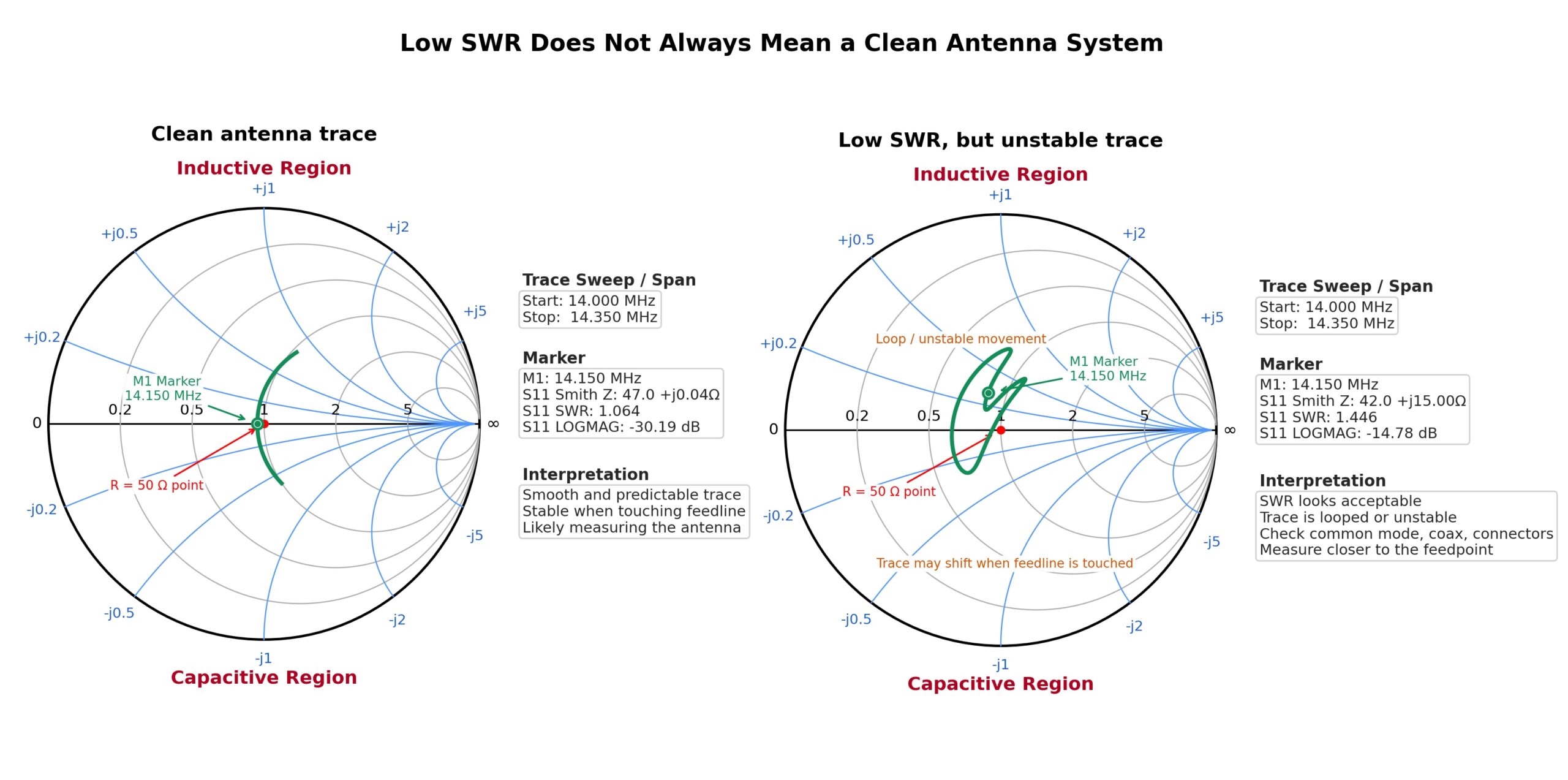
Let’s say the SWR in the shack reads 1.4:1, and we assume everything is fine. But when we bring up the Smith Chart on the NanoVNA, the trace doesn’t look clean. It forms an odd loop, shifts when we touch the coax, or changes considerably when we move the feed line just a little.
What this tells us
An antenna’s behavior should not change dramatically just because we touch the coax or slightly change the route of the feed line. If the trace on the Smith Chart changes like that, the coax is probably acting as part of the antenna. Along with carrying the signal, it may be radiating or affecting the measurement.
- An odd loop in the trace may indicate common-mode currents.
- If the trace shifts when we touch the cable, the outside of the coax shield may be radiating, or there may be a poor contact in a connector, an adapter, or another connection.
- A large difference between the impedance we measure in the shack and the impedance we measure at the feedpoint tells us the feed line is substantially transforming the impedance.
- A low SWR in the shack may be due to loss in the coax, even when the antenna itself is performing poorly.
What should we do next
- Measure as close as possible to the antenna feedpoint.
- Install a 1:1 choke balun at the feedpoint, especially on dipoles, verticals, and end-fed antennas where the coax can become part of the antenna system. With end-fed antennas, we need to choose the choke’s position carefully because the antenna needs a counterpoise, and a section of the coax itself may serve that purpose.
- Check the connectors, look for moisture, and inspect the adapters, lightning arrestors, and antenna switches.
- Repeat the measurement and compare the trace. If it becomes more stable after we add the choke and no longer shifts when we touch the cable, we’ve found a significant part of the problem.
What this means in practice: We do NOT trim the antenna just because the trace looks wrong. First, we make sure we’re measuring the antenna itself and that a radiating coax shield, a poor connection, or a faulty connector isn’t affecting the reading.
Practical example 4: An End-Fed Antenna with an unusual trace
An End-Fed antenna, especially a half-wave antenna (end-fed half-wave, or EFHW), can have a very high resistance at the feedpoint on the antenna side of the unun. The unun is an RF transformer that transforms this very high impedance, often in the 2–3 kΩ range, to a value better suited to 50 Ω coax. That’s why we use transformers with ratios such as 49:1 or 64:1, depending on the installation.
The tricky thing about an end-fed antenna is that the antenna, the unun, the counterpoise, and often the coax itself all work together as a system. That’s what makes the Smith Chart so useful. It tells us more than whether “the SWR is good or bad.” It shows us what kind of “good” or “bad” we’re looking at.
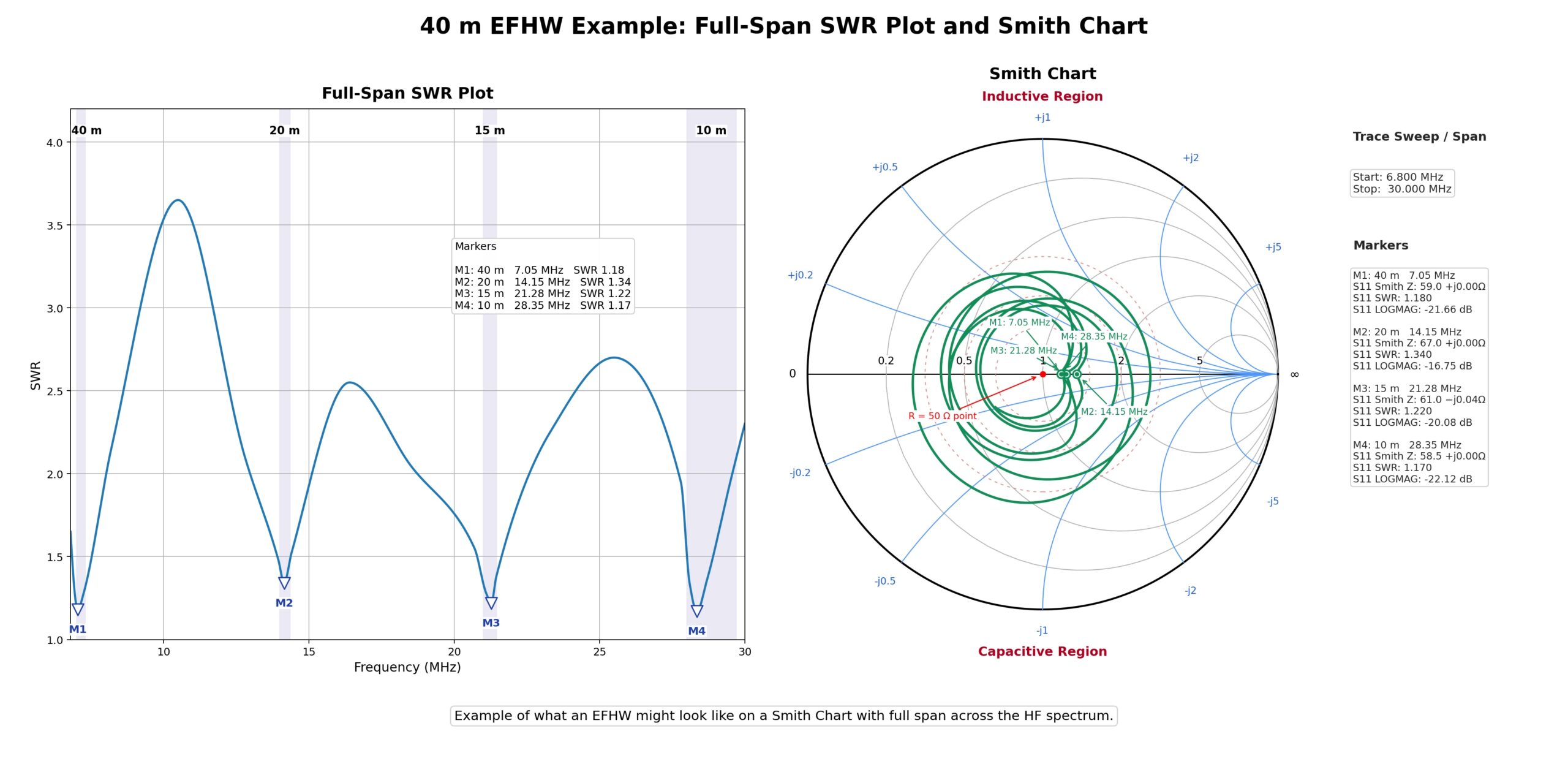
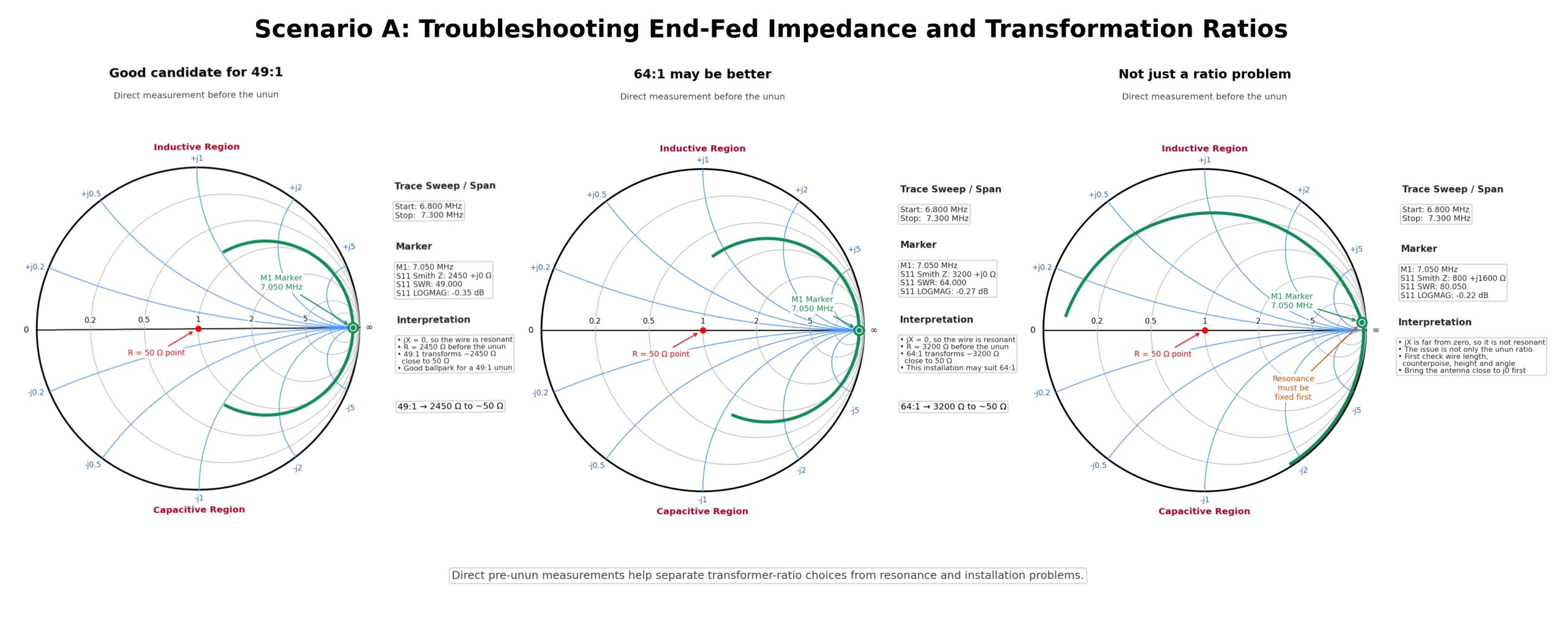
Scenario A: The trace stays far to the right and never comes close to the center
If the trace stays far to the right of the Smith Chart on the band we’re interested in, we look at the R reading at the marker. If R is much greater than 50 Ω, the resistance is high. If jX also doesn’t reach zero near the frequency we want, the end-fed antenna isn’t presenting the impedance we need for a 50 Ω system.
- If the marker is above the horizontal axis, the antenna appears inductive at that frequency.
- If it’s below the axis, the antenna appears capacitive.
- If the trace crosses the horizontal axis far to the right, the antenna may be resonant but have a very high resistance.
With an End-Fed Half-Wave antenna, this can mean that the unun isn’t transforming the impedance correctly or that this particular installation needs a different impedance ratio, for example, a 64:1 unun instead of a 49:1. It can also mean that the wire is the wrong length for the band or that the antenna lacks a suitable counterpoise.
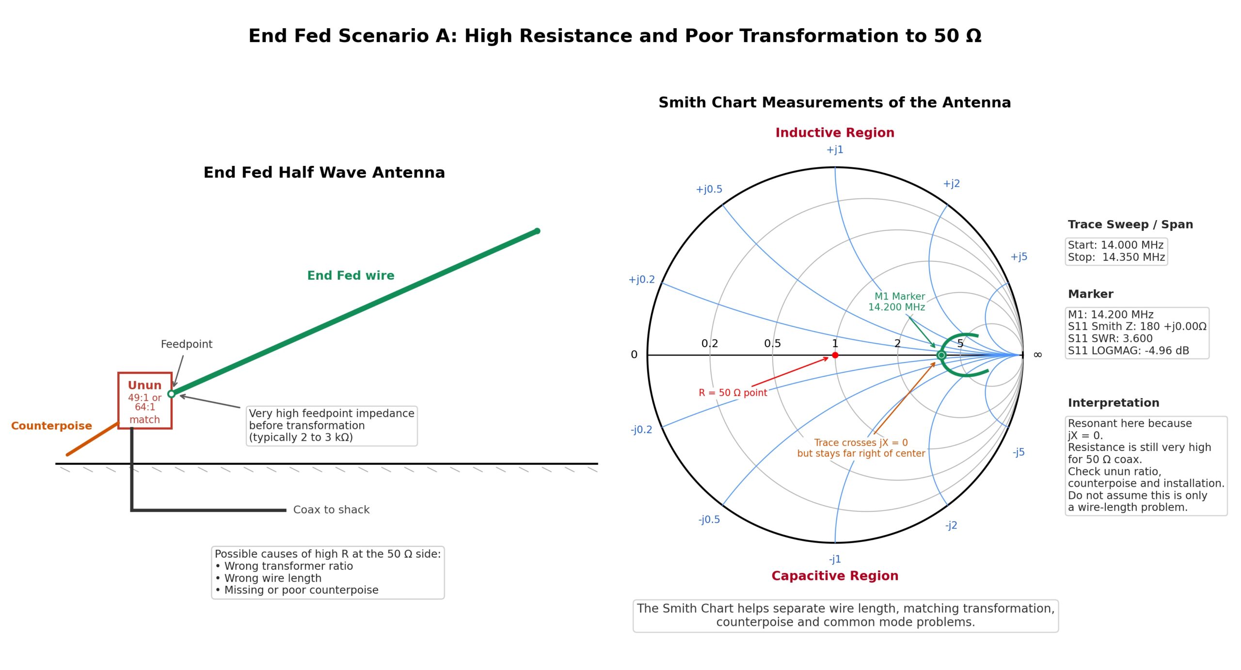
We can also measure the impedance of the wire itself before we connect it to the unun. To do that, we use the NanoVNA on the antenna side, right where the wire would normally connect to the high-impedance side of the unun.
For this measurement to mean anything, we need to make the connections correctly. We connect the antenna wire to the center conductor of the S11 port on the NanoVNA and the counterpoise or ground system to the outer conductor of that same port, the shield. If we get those connections wrong, the measurement won’t show us how the antenna actually behaves.
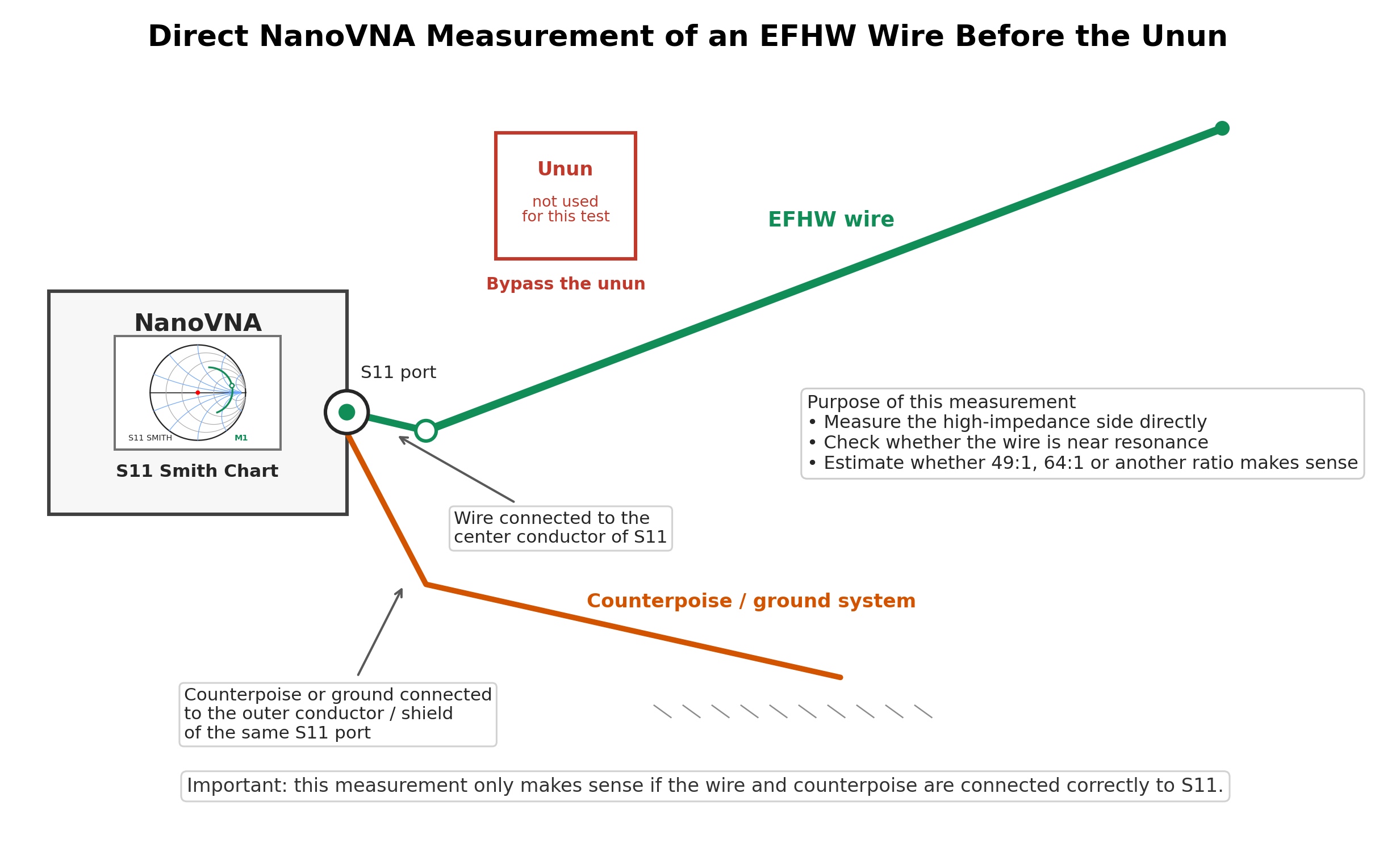
This measurement isn’t always straightforward. The counterpoise, the antenna’s height, its surroundings, the angle of the wire, and the installation as a whole all influence an end-fed antenna. The NanoVNA’s accuracy can also be limited at very high impedances. Even so, the measurement gives us a useful idea of the impedance we’re dealing with at the fundamental frequency and its harmonics.
Before we focus on the resistance reading alone, we also look at jX, the reactance. To adjust the wire length, we start with a sweep around the fundamental frequency the EFHW was cut for. We move the marker to find the frequency where jX is close to zero and the resistance R is high.
That’s how we find the antenna’s resonant frequency and compare it with the frequency we’re aiming for.
If resonance is above the frequency we want, the wire is usually electrically short, so we add a little length to bring the resonant frequency down.
If resonance falls below it, the wire is usually electrically long, so we shorten it a little to bring the resonant frequency up.
We make small adjustments and measure again until resonance is close to the frequency we want, keeping the counterpoise and the rest of the installation the same. In these cases, wire length is the first thing we check, because it determines where the antenna resonates. Near this high-impedance resonance, an EFHW that’s a little short for the frequency we’re measuring usually appears inductive (positive jX), while one that’s a little long appears capacitive (negative jX). That’s the reverse of what we see with a center-fed half-wave dipole or a 1/4λ vertical, which have a low feedpoint impedance.
So we adjust the wire length to bring jX as close as possible to j0. That puts us on the horizontal axis of the Smith Chart, where reactance is zero and the antenna is at resonance.
First, we bring the antenna close to resonance. Only then does it make sense to look closely at the resistance reading and what it means for the choice of unun transformation ratio. If the reactance is close to j0 but the impedance we see on the Smith Chart is well outside the range we’d expect, the length of the wire may no longer be the problem. We may need a different transformation ratio for the unun, a better counterpoise, or a change in how the antenna is installed, such as moving the wire, changing its height, or adjusting its angle. The aim is to bring the antenna’s impedance closer to a value the unun can properly transform to 50 Ω.
The idea is simple. The unun’s impedance ratio tells us roughly what antenna impedance it will transform to a value close to 50 Ω:
Zantenna ≈ Z50Ω × impedance ratio
In practice, that gives us:
50Ω × 49 ≈ 2,450Ω
50Ω × 64 ≈ 3,200Ω
In simple terms, a 49:1 unun is theoretically a better fit when the end-fed antenna presents an impedance of about 2,450 Ω near resonance, while a 64:1 unun is a better fit when the impedance is closer to 3,200 Ω. Other, less common ratios include 56:1 and 70:1, depending on the design of the unun and the installation.
The Smith Chart helps us see whether the high impedance of the wire, measured before the unun, falls within a reasonable range for the ratio we are using. In other words, it helps us judge whether the transformed impedance can come close to 50 + j0 Ω, or whether the unun ratio is a poor fit for that particular installation.
Scenario B: The trace changes when we touch the coax
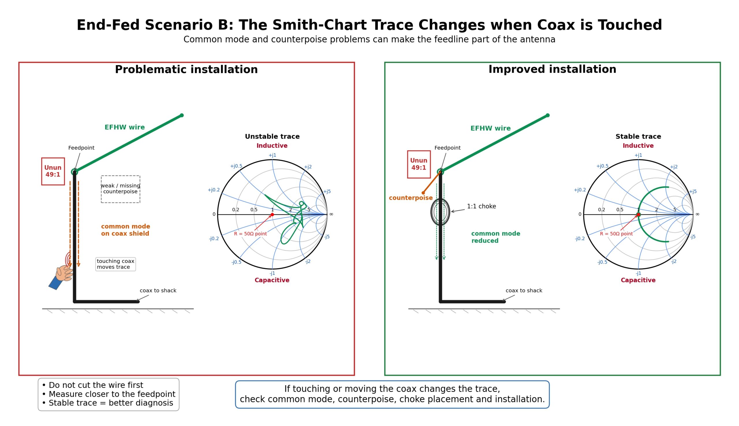
If the trace changes considerably when we touch the feed line or reroute the coax, the coax is acting as part of the antenna. This is very common in end-fed installations that lack a suitable counterpoise or choke.
- Simply trimming the wire won’t solve this.
- First, we add or adjust the counterpoise.
- Then we try a 1:1 choke at a suitable point along the feed line.
- We measure again to see whether the trace is more stable.
Scenario C: The SWR is low only when the coax is very long, is a particular length, or follows a particular route
If the SWR looks low only when the coax is very long, is a particular length, or follows a particular route, that alone doesn’t mean that the antenna is properly matched.
The length of the feed line affects the impedance our instrument sees in the shack. At the same time, a long run of coax attenuates the reflected power, which can make the SWR reading in the shack look lower than it is at the unun.
On the Smith Chart, we see the trace change position or shape depending on where we measure and how long the coax is. In the shack, we may see what looks like a good match near 50 Ω, while a measurement directly at the low-impedance side of the unun reveals the actual mismatch.
In other words, the coax doesn’t fix the antenna. It transforms the impedance we see and can hide the problem.
What should we do next
- Record SWR, R + jX, and the Smith Chart trace in the shack, with the entire feed line in place.
- Repeat the measurement directly at the unun, where the coax connects.
- Compare the two traces to see whether the coax is transforming the impedance or hiding the actual mismatch.
- If the antenna isn’t properly matched at the feedpoint, adjust the length and position of the wire, the counterpoise, the overall installation, and, if needed, the unun’s impedance ratio.
- If the trace changes when we touch the feed line, address the common-mode current with a suitable counterpoise and choke.
- Finish tuning only when the measurement at the unun feedpoint shows a satisfactory impedance and low SWR.
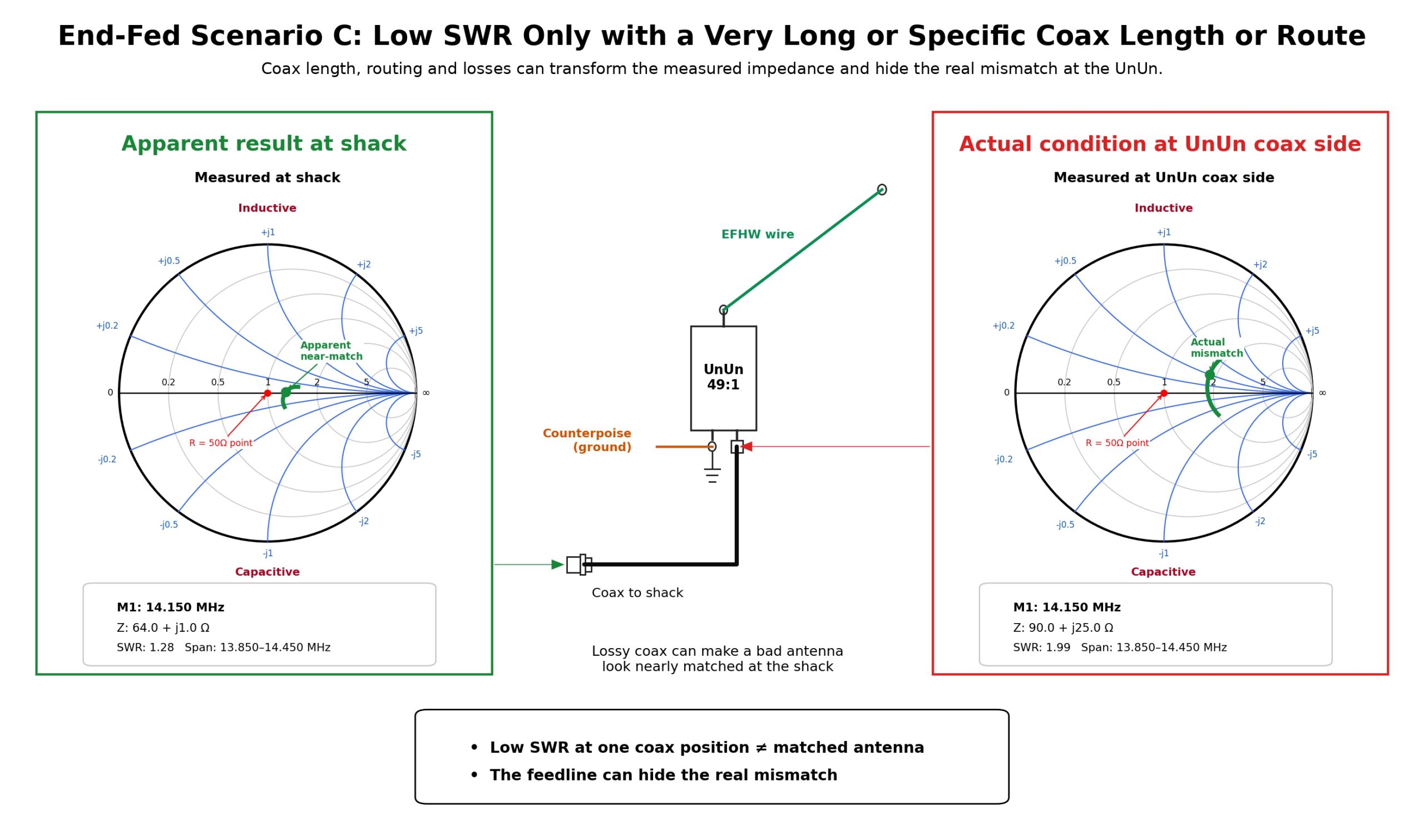
With an End-Fed antenna, the Smith Chart helps us tell three different problems apart: incorrect wire length, a poor match, and common-mode current. An SWR reading alone leaves all three looking alike.
The role of Coaxial cable
Coaxial cable is more than a simple “wire” that carries RF from the shack to the antenna. It is a transmission line. A transmission line or feed line is a cable or a system of conductors that carries RF energy. How it behaves depends on its length and on the frequency and phase of the signal.
The line has a characteristic impedance, usually 50 Ω in transmitting systems. Characteristic impedance is different from the resistance we measure with a multimeter. It describes how the cable behaves when it carries an electromagnetic wave at radio frequencies.
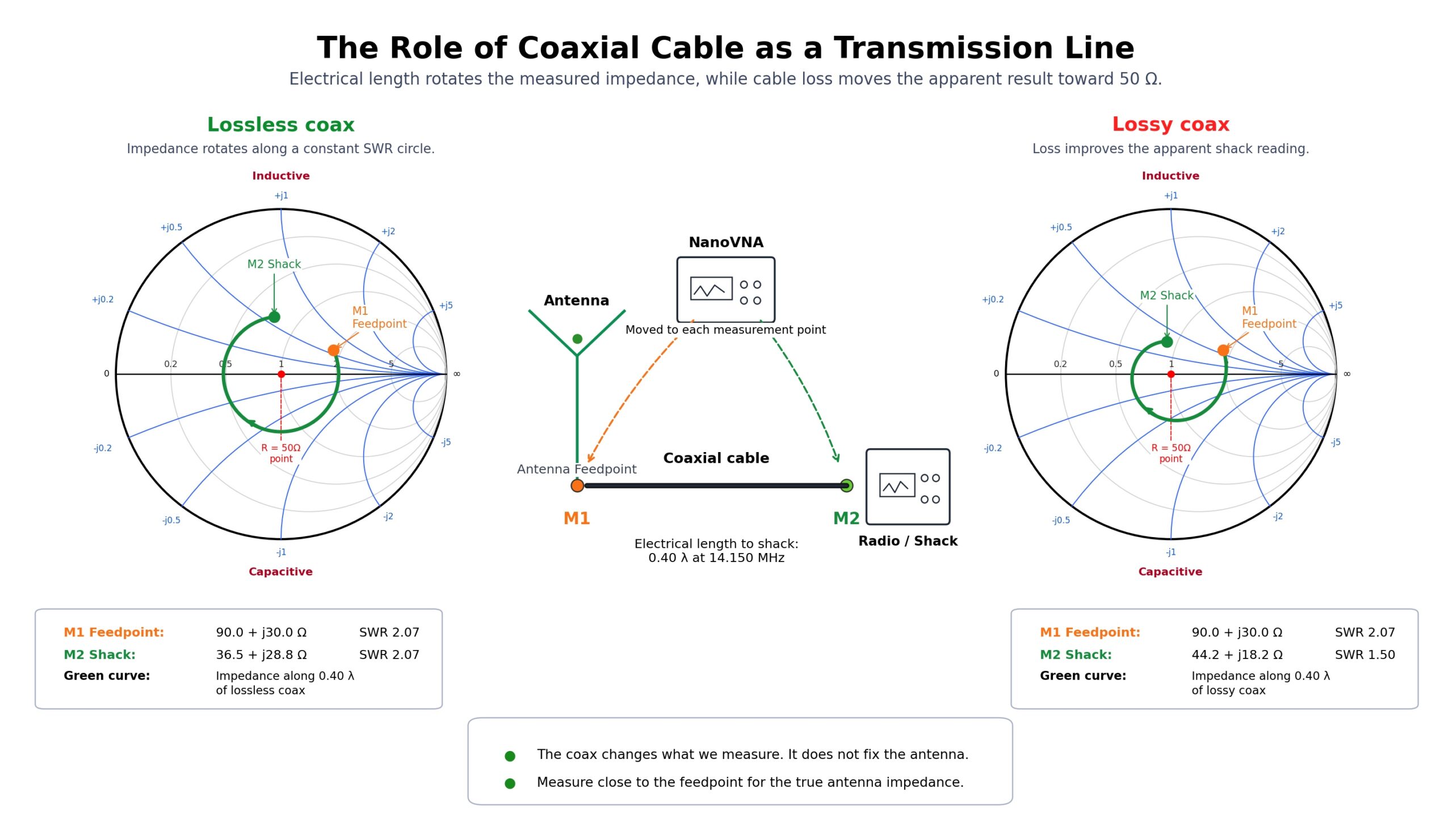
Here’s a common trap that confuses many radio amateurs. The length of the coax can transform the impedance we see in the shack. In other words, it can make the antenna look different on the NanoVNA or the SWR meter. But that doesn’t mean we’ve fixed the antenna.
On an ideal, lossless line, the SWR stays the same along the entire length of the line. What changes is the impedance we see at each point along it. This happens because the phase changes. Phase tells us “where the RF wave is” in its cycle as it travels along the cable. On the Smith Chart, we see this as a rotation around the center.
In practice, real cables have losses. Those losses can make SWR in the shack look better than it actually is at the antenna because they also attenuate the reflected wave. The reflected wave carries the portion of the power that the antenna didn’t “absorb” back toward the transmitter.
Why doesn’t changing the feed line “tune” the antenna?
We often hear operators say their antenna “started working properly” after they changed the length or type of feed line. We need to be careful about drawing that conclusion.
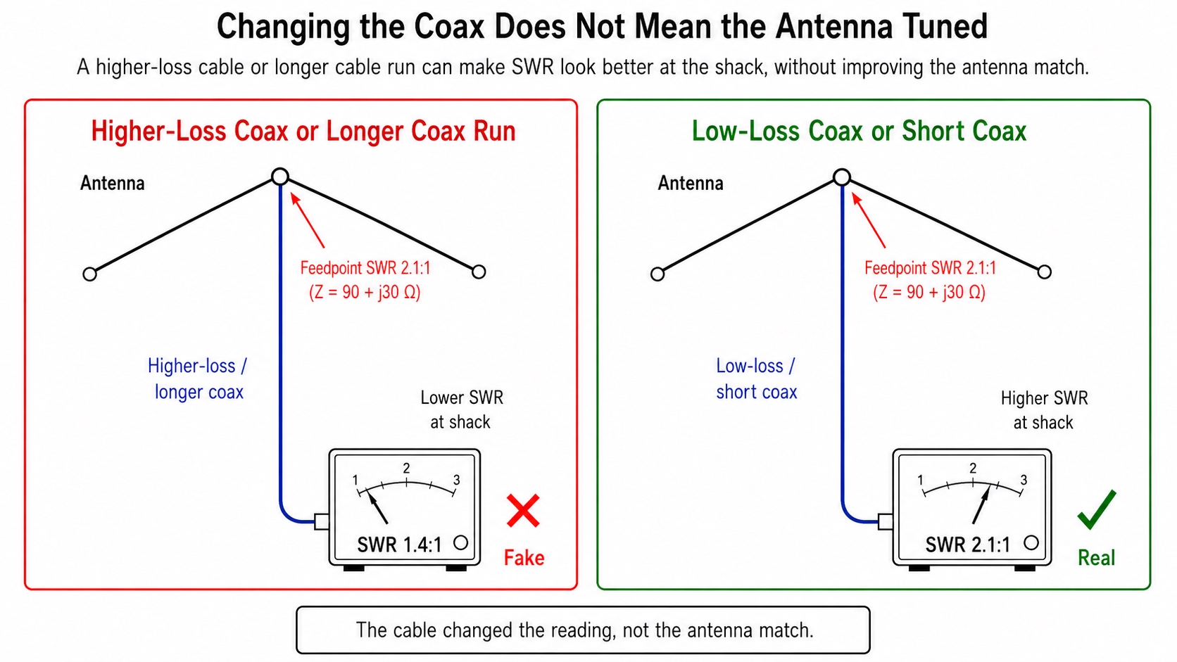
Changing the length or type of coax can change the reading we see in the shack. The SWR meter may give us a better reading. The point or trace on the Smith Chart may also move to a more favorable position. But that does not mean the antenna is now resonant or that it has started radiating better. It doesn’t mean the mismatch at the feedpoint has disappeared, either.
By mismatch, we mean that the antenna’s impedance is a poor match for the 50 Ω system. When we change the feed line, we effectively change the point from which we “look at” the antenna through that line. The same problem can still be there at the feedpoint and look different from the shack.
The right approach is to adjust the antenna as well as we can first, taking our measurements at the feedpoint. Then we check how the whole system behaves from the shack.
There’s something else worth knowing. A shorter run of coax or a lower-loss cable gives us a more accurate picture of what’s happening at the antenna. So it shouldn’t surprise us if the SWR in the shack goes up after we shorten the feed line or replace RG-58 or RG-213 with a lower-loss cable such as LMR, Aircell, or a comparable cable from Messi & Paoloni.
The old cable attenuated the reflected wave more, either because it was longer or because it had higher losses. That could make the SWR in the shack look better than it actually was at the antenna feedpoint. A shorter or lower-loss cable doesn’t create the mismatch. It simply attenuates the signal less, giving us a clearer picture of the actual match at the antenna.
Therefore, if SWR at the shack goes up after switching to shorter or lower-loss coax, don’t assume the new cable is at fault. Measure the antenna again at its feedpoint. If that measurement confirms a mismatch, adjust the antenna itself so that it resonates at the desired frequencies on the bands of interest and presents a good match to 50 Ω.
What this means in practice: If we want to know what the antenna is actually doing, we measure as close as possible to its feedpoint. When we measure through a long run of coax, what we see is the entire system; ie., the antenna and the feed line together, and not the antenna alone.
What an antenna tuner actually does
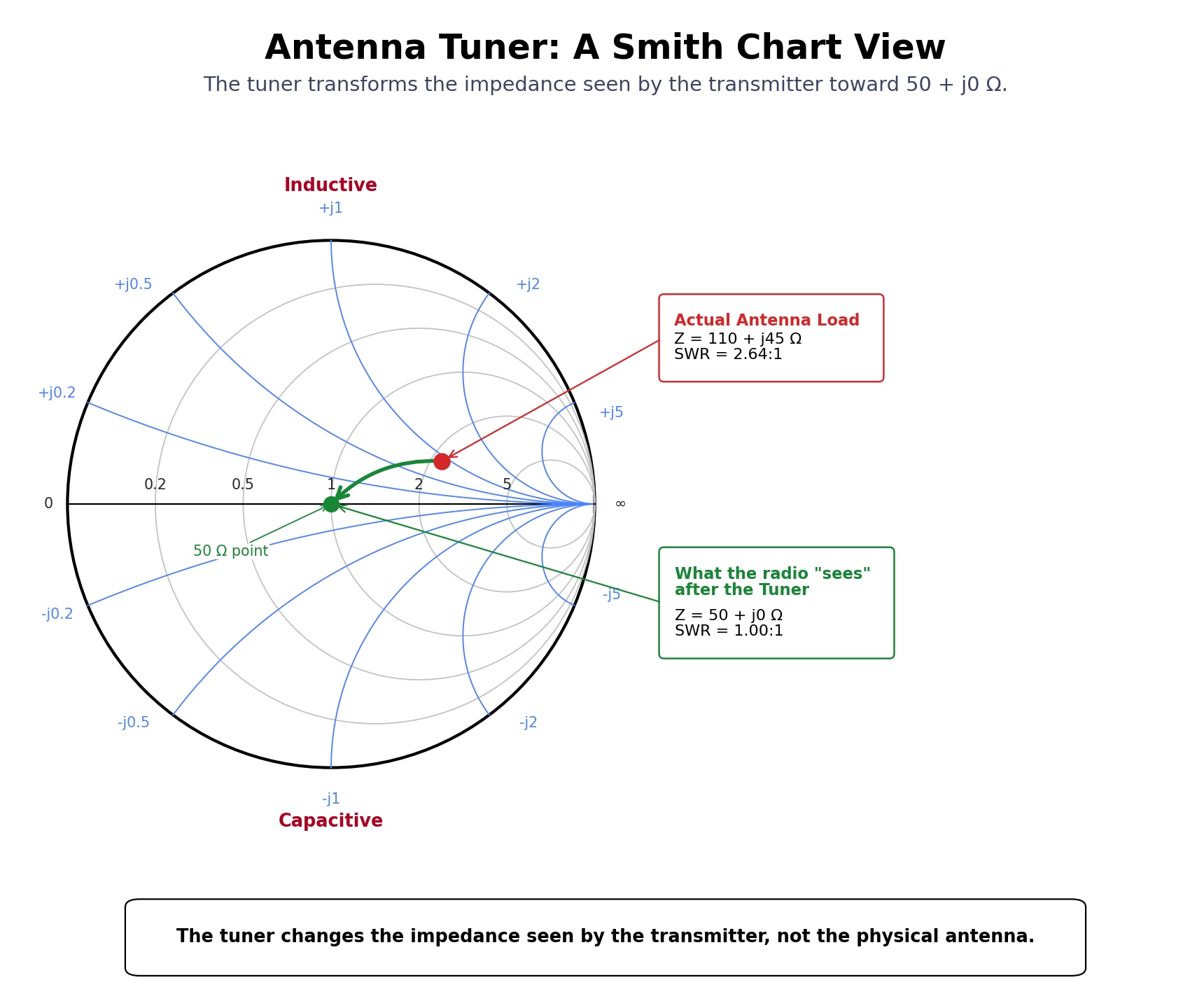
An antenna tuner doesn’t change the antenna. It doesn’t shorten it, lengthen it, or bring the antenna itself into resonance. What it does is transform the impedance the transmitter sees, so the transmitter operates into a safer, more suitable load, usually close to 50 Ω.
On the Smith Chart, the tuner’s job is to move the operating point toward the center. If the antenna appears inductive, the tuner introduces the appropriate capacitive reactance or uses a combination of components to achieve the match. If the antenna appears capacitive, it introduces the appropriate inductive reactance or uses a combination of components. If the resistive part of the impedance differs from 50 Ω, the tuner transforms it toward 50 Ω.
You don’t need to know the tuner’s internal circuit to understand the point. The tuner does not fix the antenna. It fixes the match the transmitter sees.
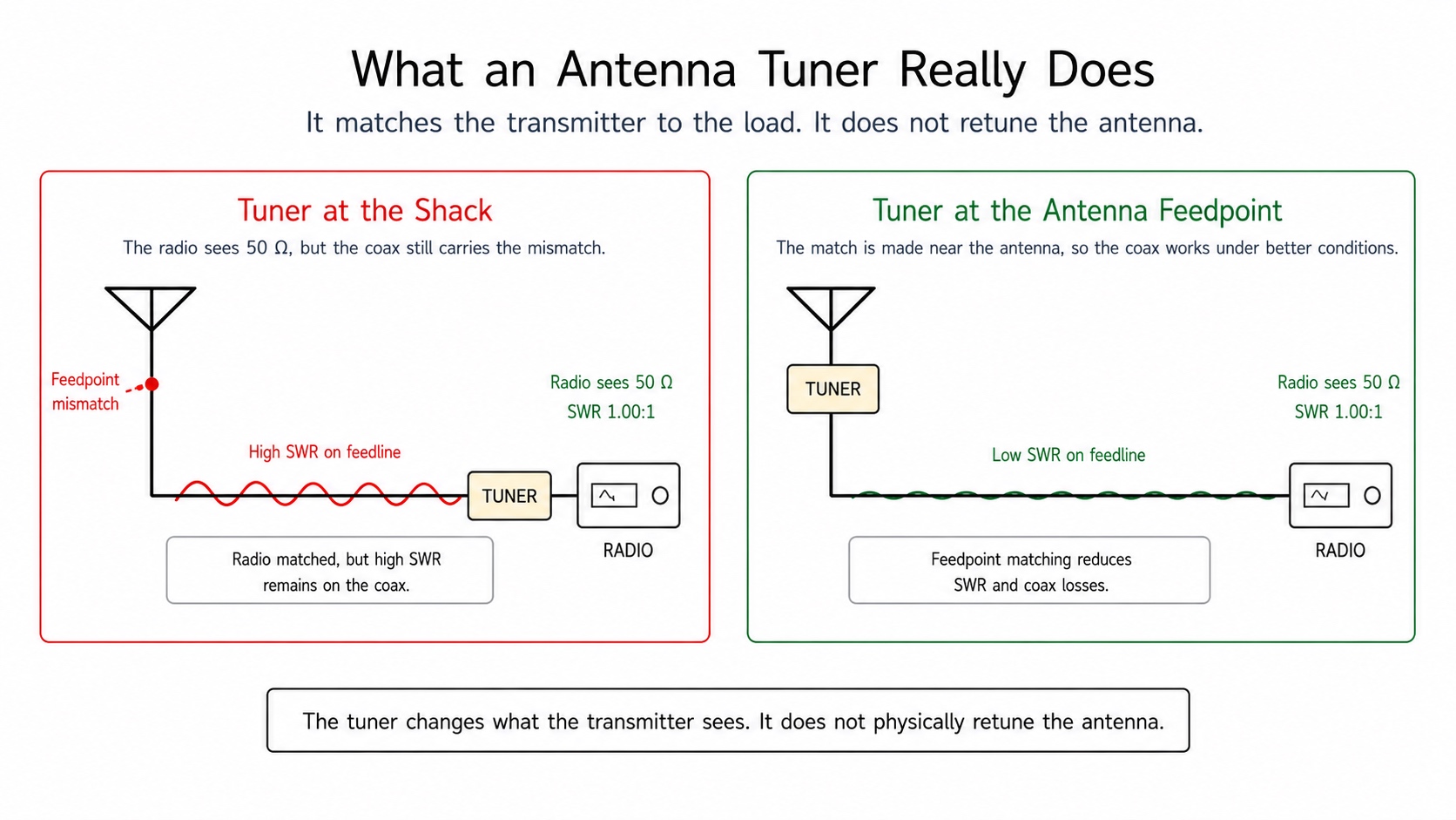
In practice, the tuner protects the transmitter and allows it to operate over a wider range of frequencies. That doesn’t mean the antenna has become efficient. If the mismatch is large and the tuner is in the shack, high voltages, high currents, and the losses they cause can still be present along the feed line.
That is why, whenever possible, the best place to match the antenna is close to the antenna itself. This reduces losses in the feed line and helps the system work better.
Common mistakes when reading the Smith Chart
Mistake 1: Looking only at SWR
SWR (standing wave ratio) is useful, but it does not tell the whole story. It tells us how severe a mismatch is without telling us what caused it. Two different impedances can give similar SWR readings yet call for entirely different adjustments. The Smith Chart shows the impedance trace across the sweep, along with the R and jX readings, so we can see how the match changes over the full frequency range. The shape of the trace and the path it follows give us a clearer picture of how the antenna or load behaves.
Mistake 2: Assuming that low SWR means the antenna is efficient
An antenna can have a low SWR even when the system has substantial losses, poor ground conditions or grounding, an inadequate counterpoise, feed line losses, or other problems. Take a dummy load, for example. It radiates virtually nothing and converts almost all the power into heat, yet it presents a perfect SWR. A low SWR mainly tells us that the transmitter sees a load it can work with. It doesn’t automatically mean the antenna radiates well, the system is efficient, or the power is going where we want it to go.
Mistake 3: Assuming that 50 Ω always means resonance
If R reads 50 Ω but jX is appreciable, the antenna is not at resonance. To determine whether it’s resonant, look at jX as well. The transmitter may see a reasonably well-matched load, but the system being measured can still be capacitive or inductive. In other words, it can still have reactance even when R is close to 50 Ω. For the antenna to be at or near resonance, jX must be at or near zero.
Mistake 4: Assuming that high SWR always means the antenna is not tuned
High SWR does not always mean the antenna is out of resonance. Take a reading of Z = 200 + j0 Ω, for example. Here jX is zero, so the antenna is resonant. The problem is that R is 200 Ω, a long way from 50 Ω, so the antenna is a poor match for the 50 Ω system. What’s needed here is an impedance transformation, for example, with a suitable 4:1 balun, an unun, or another matching network. There may be no need to modify the antenna itself or change its dimensions.
Mistake 5: Measuring from the shack and assuming the reading shows only the antenna
If there’s a long run of coax between the NanoVNA and the antenna, along with connectors, switches, lightning arrestors, or other components, the measurement includes all of them. A reading taken in the shack shows how the entire system behaves. That measurement has its place because it shows what the transmitter sees, but it is important to know exactly what is being measured. To find out whether the antenna itself is behaving as it should, measure at its feedpoint as well, and not just from the shack. Comparing the two readings helps pinpoint whether the problem is in the antenna or somewhere along the signal chain between the antenna and the shack.
Mistake 6: Trimming the antenna before understanding the shape of the trace
If the trace looks strange, forms odd loops, is unstable, or changes when the feed line is touched or moved, antenna length may not be the problem. The cause could be common-mode current, a poor connection, poor grounding, or a fault in the balun, the feed line, or elsewhere in the installation. Don’t start by modifying the antenna. First, try to isolate the problem.
This is where the Smith Chart really proves its worth. It shows us more than an SWR curve or a single impedance reading. It shows how the antenna or load behaves electrically across the frequency range we’re measuring. That lets us see what needs correcting or improving, instead of resorting to trial and error and blindly trimming or modifying the antenna before we know whether it’s actually the source of the problem. A mistake made on the antenna itself, especially once it has been cut, may be quite difficult to correct.
Video recap: From the antenna feedpoint to the shack
In the examples throughout this guide, we looked at one part of our antenna system at a time. The video below, Antenna Matching Explained: Resistance, Reactance, and SWR, closes the practical part of the guide by bringing together almost everything we’ve learned. We start with R and jX at the feedpoint. We see how much of the power is radiated and how much is lost as heat, and how a dipole’s reactance passes through zero as we adjust its length and bring it into resonance.
We then see what the relationship between the reflection coefficient Γ and SWR looks like on the Smith Chart. When we change the length of a lossless coaxial line, the marker moves around a circle of constant SWR. With loss in the coax, the marker moves closer to the center and the SWR reading in the shack looks better, even though the antenna is still the same. Finally, we see how a matching network brings the point to the center of the chart and why it matters whether we match the antenna in the shack or at the feedpoint.
A quick glossary to make sense of the jargon
Impedance: The overall “resistance” an RF load presents. It has two parts, R and jX, written together as Z = R + jX.
R: The real, or resistive, part of impedance. It behaves like ordinary resistance and accounts for power that is radiated or lost as heat.
X: Reactance. It tells us whether the antenna behaves like an inductor or a capacitor. Positive X indicates inductive behavior. Negative X indicates capacitive behavior.
jX: The way reactance is written in RF calculations. There’s no need to do the math when using the NanoVNA. What matters here is whether the reactance is positive, negative, or close to zero.
Complex number: A number with two parts. In this guide, it appears in the form R + jX. R is the resistive part, and jX tells us whether the load behaves like an inductor or a capacitor. You don’t need to know complex algebra to use the Smith Chart.
Normalization: Expressing an impedance value relative to the system’s reference impedance, usually 50 Ω. This allows the NanoVNA to display different impedance values on the same Smith Chart.
Phase: Where an RF wave is in its cycle as it travels, expressed in terms of time or electrical angle. With a mismatched antenna, the length of the coax can change the impedance we see in the shack because it affects the phase difference between the wave traveling toward the antenna and the wave reflected back from it.
Magnitude: When we talk about the magnitude of Γ, we mean how strong the reflection is, regardless of its phase. On the Smith Chart, this corresponds to the point’s distance from the center.
RF load: Anything connected to the transmitter output or the end of a transmission line that “receives” the signal. It could be an antenna, a dummy load, a tuner, or a matching network.
Resonance: The point where the reactance is at or near zero. At resonance, the antenna appears neither capacitive nor inductive. Its resistance can still be something other than 50 Ω.
A 50 Ω match: The condition in which the load the transmitter sees is close to 50 + j0 Ω. That makes the transmitter happy, but it doesn’t by itself tell us whether the antenna is efficient.
SWR: Standing wave ratio. It tells us how well the load matches the line. It’s a useful reading, but it gives only part of the picture. A low SWR doesn’t necessarily mean the antenna is good or efficient.
Γ: The reflection coefficient. It describes how much of the signal is reflected back because of an impedance mismatch. In practice, the NanoVNA uses it to draw the Smith Chart, but what we mainly see is how far the point lies from the center.
Characteristic impedance: The impedance an RF transmission line is designed for. In most amateur radio systems, it is 50 Ω. You can not measure it simply by connecting a multimeter across the cable.
Common-mode current: Current flowing on the outside of the coax shield. It can cause the cable to radiate, affect measurements, and bring RF into the shack.
1:1 Choke Balun: A device that helps limit common-mode current on the coax. It doesn’t transform impedance the way a 49:1 transformer does. Instead, it acts like a brake, choking the unwanted current flowing along the outside of the coax shield.
4:1 Current Balun: An impedance transformer that, in practice, can step the impedance of a balanced load down from about 200 Ω to roughly 50 Ω to match an unbalanced feed line such as coax. It is useful when the antenna is resonant but its feedpoint impedance does not match a 50 Ω system.
Unun: An RF transformer used between unbalanced circuits, for example, where coax feeds an End-Fed antenna. Ratios such as 49:1 or 64:1 are often used to step down a very high impedance closer to 50 Ω.
Radials: Wires that provide an RF return path or serve as a ground system for many vertical antennas. They have a strong influence on efficiency, feedpoint resistance, and how stable the measurement is.
Feed line or transmission line: The line that connects the transmitter or NanoVNA to the antenna. It is usually 50 Ω coax.
Matching: The process of bringing the impedance presented by the antenna closer to the impedance of our 50 Ω system.
So, what do we take away from all this?
There’s no need to be afraid of the Smith Chart. It’s more than a theoretical diagram. It’s a practical map of how our antenna behaves.
The center shows a good match. The upper half shows inductive behavior. The lower half shows capacitive behavior. Along the horizontal axis, resistance is lower than 50 Ω to the left of center and higher than 50 Ω to the right. The distance from the center tells us how strong the reflection is.
The most important thing to remember, though, is how to recognize resonance. The main indication is that jX approaches zero. For a perfect match to a 50 Ω system, look for both conditions together: R is about 50 Ω and jX is about zero. Resonance and a perfect match often coincide, but they don’t always go hand in hand.
Once you learn to read those few features of the chart, the NanoVNA becomes more than an instrument that displays SWR. It becomes a diagnostic tool. It can show you whether to lengthen or shorten the antenna, check for common-mode current, improve the radials, inspect the coax, use a suitable matching network, or simply leave the antenna alone.
The next time you connect your NanoVNA, take a moment to look at the Smith Chart before switching to the SWR display. Without working through a single formula, you can read the trace, understand what your antenna is telling you, and decide what, if anything, needs adjusting.
And that is the real value of the Smith Chart for the Radio Amateur.
Once we learn how to read it, it stops looking like “black magic” and becomes what it was always meant to be: a practical map of what our antenna system is doing, where the problem lies, and what we need to do next.